Describing Data: Numerical Measures

Presentation on theme: "Describing Data: Numerical Measures"— Presentation transcript:

1 Describing Data: Numerical Measures
Copyright © 2015 McGraw-Hill Education. All rights reserved. No reproduction or distribution without the prior written consent of McGraw-Hill Education.

2 Learning Objectives LO3-1 Compute and interpret the 平均數 (mean), the 中位數 (median), and the 眾數 (mode). LO3-2 Compute a 加權平均數 (weighted mean). LO3-3 Compute and interpret the 幾何平均數 (geometric mean). LO3-4 Compute and interpret the 全距 (range), 變異數(variance), and 標準差 (standard deviation). LO3-5 Explain and apply 柴比雪夫定理 (Chebyshev’s theorem) and the 經驗法則 (Empirical Rule). LO3-6 Compute the mean and standard deviation of 分組資料 (grouped data). 3-*

3 LO3-1 Compute and interpret the mean, the median, and the mode.
Measures of Location The purpose of a measure of location is to pinpoint the center of a distribution of data. There are many measures of location. We will consider three: The arithmetic mean （算數平均數） The median （中位數） The mode（眾數） 3-*

4 Characteristics of the Mean
LO3-1 Characteristics of the Mean 算術平均數最常被用來衡量區位(measure of location 它 至少需要 interval scale（區間/等距尺度）. 它的主要特點為： 必須使用所有數值. 它是獨一無二的. 所有觀察值與平均數之差距的總和為零（故：平均數兩邊的觀察值與平均數的距離和相等）. 平均數＝所有觀察值的總和除以觀察值數目. . 3-*

5 母體平均數 Population Mean LO3-1
就未分組資料(ungrouped data)而言, 母體平均數乃是所有母體觀察數值的加總除以母體觀察值的數目，而得到之平均數： 3-*

6 LO3-1 Example – 母體平均數 (p.52) 在 Kentucky 州內的州際公路 I-75 有 42 個出口， 下面列出各個出口間的距離 (in miles). 為何此資料為母體 population資料? 出口間距的平均英里數為何? 3-*

7 LO3-1 Example – 母體平均數 (p.52) There are 42 exits on I-75 through the state of Kentucky. Listed below are the distances between exits (in miles). Why is this information a population? This is a population because we are considering all of the exits in Kentucky. What is the mean number of miles between exits? 3-*

8 Properties of the Arithmetic Mean
LO3-1 Properties of the Arithmetic Mean 凡資料為 interval-level 或 ratio-level data 都有平均數。 計算平均數必須使用所有資料。 平均數是獨一無二的。 觀察值與平均數的差距和為零。 3-*

9 參數(Parameter) versus 統計值(Statistic)
LO3-1 參數(Parameter) versus 統計值(Statistic) PARAMETER A measurable characteristic of a population. （母體）參數 . STATISTIC A measurable characteristic of a sample.（樣本）統計值 3-*

10 LO3-1 樣本平均數 Sample Mean 就未分組資料(ungrouped data)而言，樣本平均數乃是所有樣本觀察值的總和除以樣本數目，而得到之平均數： . 3-*

11 LO3-1 Example – 樣本平均數 (p.54) 3-*

12 平均數 (3-1)

13 平均數 : 特性 (3-2) (3-3) (3-4)

14 中位數 The Median (p.56) MEDIAN 中位數乃是將觀察值排序（由小到大）後，位於中間的那個數值 (midpoint )。
LO3-1 中位數 The Median (p.56) MEDIAN 中位數乃是將觀察值排序（由小到大）後，位於中間的那個數值 (midpoint )。 中位數(median)的特性: 每一組資料都有獨一的中位數。 它不受極端值（極大或極小值）影響，所以它是很有用的中間趨勢值。 以下3種資料（尺度）都有中位數： ratio-level, interval-level, 以及 ordinal-level data.。 即使在開放式（組下限或組上限為無窮小、或無窮大時）的次數分配中，只要中位數不在開放式的組別中，都可求出中位數。 3-*

15 open-ended frequency distribution
如：常態分配，其極大值或極小值可趨近於無窮大/小，但常態分配還是有中位數。 只要中位數不在開放組（如：組上限無窮大）中，就能找到中位數。

16 LO3-1 Examples – 中位數Median （樣本）5位大學生的年齡為： 21, 25, 19, 20, 22 重新按年齡遞增排序為： 19, 20, 21, 22, 25. 故中位數 median 為 21. 4位籃球選手的身高（單位：英吋）為： 76, 73, 80, 75 重新遞增排列如下： 73, 75, 76, 80. 故中位數 median為75.5. 3-*

17 中位數 一組按大小順序排列的資料x1,x2…xn，其中位數為位於中間位置的數值，亦即： 當n為奇數時，第 位置的數值為其中位數

18 LO3-1 眾數 The Mode (p.58) MODE The value of the observation that appears most frequently. 出現最多次的數值就是眾數 3-*

19 LO3-1 Example - Mode Using the data measuring the distance in miles between exits on I-75 through Kentucky, what is the modal distance? Organize the distances into a frequency table and select the distance with the highest frequency. 3-*

20 Example – 眾數Mode (p.59) 用Kentucky 州內I-75 出口間距的資料，請問其眾數為多少英里？
LO3-1 Example – 眾數Mode (p.59) 用Kentucky 州內I-75 出口間距的資料，請問其眾數為多少英里？ 將間距組成次數表，而後選出次數最多者為眾數。 問：眾數是否為此資料的最佳代表值？平均數呢？中位數呢？ 眾數＝1英里 平均數＝4.57英里 中位數＝3英里 3-*

21 那個參數/統計值最能表現中間位置？ 算數平均數？（受極端值影響，如前例的11、14，使得平均數偏大） 中位數？
眾數？（出現最多次者，但不保證資料一定有眾數，如：每一觀察值都只出現一次）前例中，眾數乃由ordinal分組取得，而距離為ratio尺度，眾數不能代表ratio尺度的變數。

22 Quick review: 資料的中央趨勢：算數平均數、中位數、眾數 (1) 算數平均數： 優點： 考量到一組數值中所有的觀察值 缺點：
易受極端值影響 哪些資料可以計算？ 區間尺度資料、比例尺度資料 μ？X? ＊加權平均數：(64頁） 算數平均數的特別例子，主要是考量到各數值的重要性不同。 22

23 (2) 中位數： 優點： 不易受極端值影響 缺點： 沒有考量到數值中所有的觀察點 (3) 眾數： 沒有考量所有的觀察點，而且有時沒有眾數，甚至於 有時會有兩個以上的眾數。 & 幾何平均數：計算變動量的平均（65頁）

24 Mean, Median 以及 Mode 的相對位置
LO3-1 Mean, Median 以及 Mode 的相對位置

25 加權平均數 Weighted Mean (p.64)
LO3-2 Compute a weighted mean. 加權平均數 Weighted Mean (p.64) The weighted mean of a set of numbers X1, X2, ..., Xn, with corresponding weights w1, w2, ...,wn, is computed with the following formula: 3-*

26 Example – Weighted Mean(p.64)
LO3-2 Example – Weighted Mean(p.64) The Carter Construction Company支付其26個按時計酬員工的時薪為： $16.50, $19.00, or $25.00 per hour. 其中： 14 個為 $16.50 、 10 個為 $19.00 、而 2 個為 $25.00 。 這26個員工的平均時薪為多少？ 3-*

27 幾何平均數 The Geometric Mean (p.65)
LO3-3 Compute and interpret the geometric mean. 幾何平均數 The Geometric Mean (p.65) 用於計算％變動、比例變動值、指數變動值、成長率的平均值時，極為有用。 在商業與經濟中應用極廣，因為我們通常會想知道：銷售、薪資、或某些經濟指標的平均成長％比例，如： GDP成長率 幾何平均數永遠小於等於算數平均數 3-*

28 幾何平均數: Finding the Average Rate of Return over time
LO3-3 幾何平均數: Finding the Average Rate of Return over time EXAMPLE: (p.66) The return on investment earned by Atkins Construction Company for four successive years was: 30 percent, 20 percent, -40 percent, and 200 percent. What is the geometric mean rate of return on investment? 3-*

29 幾何平均數: Finding an Average Percent Change Over Time
LO3-3 幾何平均數: Finding an Average Percent Change Over Time EXAMPLE: During the decade of the 1990s, and into the 2000s, Las Vegas, Nevada, was the fastest-growing city in the United States. The population increased from 258,295 in 1990 to 584,539 in This is an increase of 326,244 people, or a percent increase over the period. What is the average annual increase? 3-*

30 LO3-4 Compute and interpret the range, variance, and standard deviation.
離散度 Dispersion A measure of location,：如平均數、中位數，僅能衡量資料的中間趨勢值，卻不能告訴我們資料如何分布。 例如：若旅遊指南說你前面這條河平均深度3公尺，你能不多收集資料就涉水渡河嗎？可能不會，你會想知道河水深度的變異情況，再做渡河的打算。 第二個理由是：資料離散度可以用來比較兩個或多個分配的分布情況。 3-*

31 Measures of Dispersion
LO3-4 Measures of Dispersion Range 全距 Variance 變異數 Standard Deviation 標準差 3-*

32 LO3-4 Example – Range（全距） The number of cappuccinos sold at the Starbucks location in the Orange County Airport between 4 and 7 p.m. for a sample of 5 days last year were 20, 40, 50, 60, and 80. Determine the range for the number of cappuccinos sold. Range = Maximum value – Minimum value = 80 – 20 = 60 3-*

33 Computing the Variance
LO3-4 Computing the Variance Steps in computing the variance: Step 1: Find the mean. Step 2: Find the difference between each observation and the mean, and square that difference. Step 3: Sum all the squared differences found in Step 2. Step 4: Divide the sum of the squared differences by the number of items in the population. 3-*

34 變異數Variance and 標準差Standard Deviation
LO3-4 變異數Variance and 標準差Standard Deviation VARIANCE The arithmetic mean of the squared deviations from the mean.與平均數之差距平方和除以母體個數 STANDARD DEVIATION The square root of the variance. 變異數與標準差皆為正數(nonnegative)，若全部觀察值都為相同值，則變異數與標準差都＝0 。 若母體值都很接近其平均數，則變異數與標準差的數值會很小。 若母體值距離平均數很遠（離散度大），則變異數與標準差的數值會很大。 變異數使用全部母體數值，而全距僅用到最大值與最小值，因此變異數優於全距。 3-*

35 LO3-4 Example – 變異數與標準差 The number of 罰單(traffic citations) issued during the last twelve months in Beaufort County, South Carolina, is reported below: What is the population variance? Step 1: Find the mean. 3-*

36 Example –變異數與標準差 Continued
LO3-4 Example –變異數與標準差 Continued What is the population variance? Step 2: Find the difference between each observation and the mean of 29, and square that difference. Step 3: Sum all the squared differences found in Step 2. Step 4: Divide the sum of the squared differences by the number of items in the population. 3-*

37 LO3-4 樣本變異數 Sample Variance 3-*

38 樣本變異數的自由度＝n-1 求樣本變異數，先求樣本平均數，再計算各樣本值與平均數之差的平方，再計算離均差平方的算術平均數。此時自由度因為計算樣本平均值而去掉1個，故而最後計算平方和的平均數，不能除以n，必須除以自由度。（因為失去的1個自由度的數值，會隨著平均數公式而變動，不能用來計算平方和的平均值） 自由度：樣本中能獨立/自由變化的個數

39 樣本變異數的自由度＝n-1 想像：從母體中抽出3個樣本，如果樣本的平均值固定為3，則只有2個樣本數值可以自由變化，一旦2個樣本數值已經被決定，第3個樣本的數值就被迫固定，不能改變。故而，真正的「變量」只有2個。 樣本的變異數必須用到樣本平均數 ͞x 來計算。 ͞x 在抽樣完成後便已確定，所以大小為n的樣本中只要n-1個數確定了，第n個數就能使樣本符合 ͞x 的數值。也就是說，樣本中只有n-1個數可以自由變化，只要確定了這n-1個數，標準差也就確定了。這裡，平均數 ͞x 就相當於一個限制條件，由於加了這個限制條件，樣本變異數的自由度為 n-1。

40 變異數—母體 (3-9)

41 變異數—樣本 (3-11)

42 變異數 (3-12)

43 LO3-4 Example – 樣本變異數 (p. 76) The hourly wages for a sample of part-time employees at Home Depot are: $12, $20, $16, $18, and $19. The sample mean is $17. What is the sample variance? 3-*

44 樣本標準差 Sample Standard Deviation
LO3-4 樣本標準差 Sample Standard Deviation 3-*

45 柴比雪夫定理 Chebyshev’s Theorem
LO3-5 Explain and apply Chebyshev’s theorem and the Empirical Rule. 柴比雪夫定理 Chebyshev’s Theorem The arithmetic mean biweekly amount contributed by the Dupree Paint employees to the company’s profit-sharing plan is $51.54, and the standard deviation is $7.51. At least what percent of the contributions lie within plus 3.5 standard deviations and minus 3.5 standard deviations of the mean? 3-*

46 表3.3 各種不同k值之Chebyshev定理的應用
區間 落於該區間內觀測值的比例 1 至少為0(至少0%) 2 2.5 3

47 柴比雪夫定理 Chebyshev’s Theorem
不論資料為何種分配，至少有(1-1/k2)的資料落在距離平均數 ±k 個標準差的範圍內，k>1。 i.e. Prob(|X-μ|≦kσ) ≧1-(1/k2) or Prob (μ-kσ ≦X ≦ μ+kσ) ≧1-(1/k2) 或 Prob(|X-μ| ≧ kσ) ≦ (1/k2) i.e. Prob (X≦μ-kσ or X ≧μ+kσ)≦(1/k2)

48 經驗法則 The Empirical Rule
LO3-5 經驗法則 The Empirical Rule 3-*

49 經驗法則 若為對稱鐘形分配，平均數左右1個標準差範圍內，約有68％的觀察資料，平均數左右2個標準差範圍內，約有95％的觀察資料，平均數左右3個標準差範圍內，約可涵蓋所有資料（99.7％的觀察資料）。

50 經驗法則 當資料分配呈鐘形形狀(bell-shaped)時，亦即為對稱分配，則 約有68%的觀測值落於 的區間內。
約有68%的觀測值落於 的區間內。 約有95%的觀測值落於 的區間內。 約有99.7%的觀測值落於 的區 間內。

51 表3.4 Chebyshev定理與經驗法則之比較
區間 Chebyshev定理 經驗法則 至少0% 約68% 至少75% 約95% 至少89% 約99.7%

52 分組資料(Grouped Data)的算數平均數
LO3-6 Compute the mean and standard deviation of grouped data. 分組資料(Grouped Data)的算數平均數 3-*

53 分組資料（若無法還原成原始資料時） 計算：各組資料的總和＝各組次數*組中點 假設：各組資料都是均勻分布，組中點＝該組的算數平均數。
故：分組資料的平均＝各組總和的加總/總次數

54 分組資料：用組中點求平均數 If then so

55 Example - The Arithmetic Mean of Grouped Data (p.81)
LO3-6 Example - The Arithmetic Mean of Grouped Data (p.81) 在第二章中，我們做了次數分配表，列出Applewood Auto Group所售出的180輛車的利潤，如右表所示：若不管原始資料，單以此表計算每輛車的平均利潤，該如何計算？ 3-*

56 Example – 用分組資料計算平均值 (p.82)
LO3-6 Example – 用分組資料計算平均值 (p.82) 3-*

57 Example - Standard Deviation of Grouped Data
LO3-6 Example - Standard Deviation of Grouped Data Refer to the frequency distribution for the Applewood Auto Group data used earlier. Compute the standard deviation of the vehicle profits. 3-*

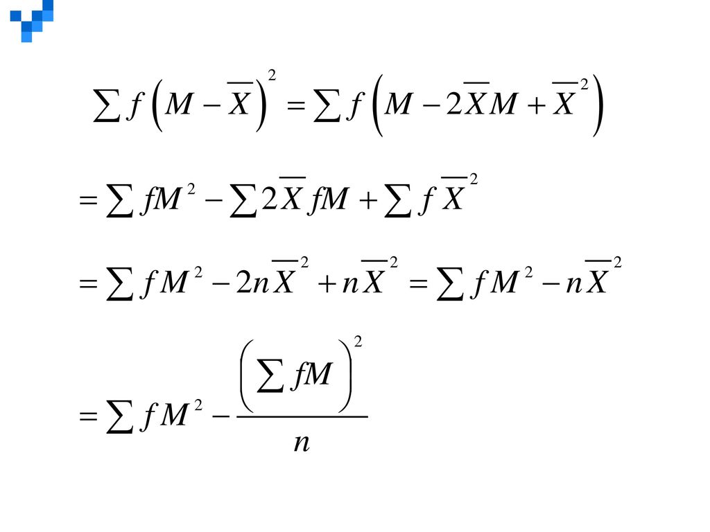
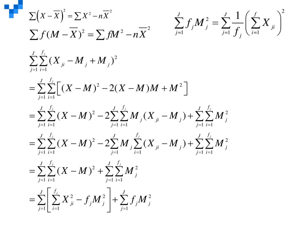
58 分組資料：求樣本變異數的2個公式

59

60

61