Measures of location and dispersion

Presentation on theme: "Measures of location and dispersion"— Presentation transcript:

1 Measures of location and dispersion
定義 1. What is the general shape or distribution of the data? 資料分佈的形狀? 2. Where is the center of the data, or what is the average value of the data ? 資料的中心點?平均值為何? 3. How dispersed, or spread out, are the data ? 資料分散的程度如何? 除了以圖形來瞭解，我們也可以用某些具體數量來回答上述問題。

2 Parameters 定義 Numbers that describe population characteristics are called parameters. 描述母體的表徵數稱之為母數（或參數）如母體平均數，母體變異數、母體比率等。 Much of the field of statistics is devoted to drawing inferences from a sample concerning the value of a population parameter.

3 Estimate估計值 and Estimator估計量
定義 從樣本中計算得來，用來估算一未知母數的統計量稱為估計量值(estimates)，用來計算估計值的計算公式稱為估計式(estimator) Values calculated from a sample of data that are used to estimate population parameters are called estimates估計值. The formula used to calculate an estimate is called an 估計式(estimator.

4 Estimate估計值 and Estimator估計量
定義 An estimator is a function, whereas an estimate is a specific value. 估計量為一數學函數，而估計值為一特定的數值。

5 符號 xi 一般以x, y, z來作為變數的代號。例如可以將出生年這個變數用x來表示。
xi變數右下角的小注標(subscript)，用來標示觀察值的序號，表示為第i個觀察值。如資料中第三位受訪者的出生年為x3 = 41

6 Summation Notation 基本運算複習
定義 以大寫的N來表示母體中觀察值的總個數，以小寫的n來表示樣本中的觀察值總數。 以小寫a, b, c來表示常數。 將母體當中，所有觀察值加總，可以表為： 從x1加到xN Σ英文讀做summation sign

7 基本運算複習 定義 規則一：加總運算遇到刮號可以直接展開 兩個變數相加的和 =先將每個變數單獨加總之後，再相加。 12+16=28

8 基本運算複習 定義 規則二：Σ遇到常數項可以直接將常數提到Σ外

9 基本運算複習 定義 規則三：Σ內若只有常數c，等於將該常數加N遍，其和為N × c

10 基本運算複習 定義 規則四：ΣΣ的運算方式：

11 基本運算複習 規則五：任何在Σ內，但不因Σ的注標而變化的數值，皆可當成常數來處理。 沒有注標，不隨i而變化 y沒有i注標，不會隨i而變化
定義 規則五：任何在Σ內，但不因Σ的注標而變化的數值，皆可當成常數來處理。 沒有注標，不隨i而變化 y沒有i注標，不會隨i而變化

12 基本運算複習 定義

13 基本運算複習 定義 是否等於

14 基本運算複習 定義 簡化原則：summation遇到多項式的乘冪，一般先將乘冪乘開，然後再將summation括弧展開。

15 測量集中趨勢--Population Mean
定義 母體平均值以希臘字母的μ(讀成mu)表示，計算式 : 在特定的時空內，母體平均值只有一個，是特定的一個數值，因此為一常數。 大N通常代表母體的個數

16 樣本平均值Sample Mean 給定 n 個樣本觀察值， x1, x2, … xn, 樣本平均值（讀做x bar)定義為:
每一個特定樣本僅有一個平均值，就一特定樣本而言，樣本平均值是一個常數。例如本班同學的平均身高為一特定值。 但不同樣本會有不同的平均值，因此樣本平均數也可以是一個變數。如不同班級（樣本不同）有不同的平均身高。

17 Sample Mean 初統中的證明題，經常用到這個式子，請牢記。 全體觀察值的總和 = 樣本平均值乘以樣本數
定義 初統中的證明題，經常用到這個式子，請牢記。 全體觀察值的總和 = 樣本平均值乘以樣本數 樣本平均值可以想成是每一個觀察值的代表性數值(typical value)。

18 間斷性分組資料的算數平均數 定義 n

19 連續性分組資料的算數平均數 定義

20 連續性分組資料的算數平均數 分組資料中若有開放式的組界，由於該組的組中點無法決定，因此其平均數亦無法計算。 Name Income f A
3 ~ 4 23 B 5 12 C 6 34 D 7 E 7以上 32 Average ？？

21 平均值的特質 平均值為資料的平衡點(center of gravity) 各觀察值與平均數間的差的總和最小 各觀察值與平均數之差的平方和最小
缺點為易受極端值的影響。

22 重力的平衡點 Center of gravity

23 資料的平衡點 平均值是使所有觀察值與此點的距離和最小的一個平衡點。

24 算數平均數的性質 各個觀察值與平均數差的總和為0 證明 同理，分組資料：

25 觀察值與平均數之差的平方和最小 各個觀察值與平均數差的平方和為最小 常數 等於0 大於等於0

26 平均值易受極端值的影響 平均值容易受到極端值(outlier)的影響，若資料中有過大或過小的觀察值時，不要以平均值來代表集中趨勢。 Name
Income A 3 B 4 C 5 D E 60 Average 15

27 平均值可以進行代數演算 設x1, x2, x3, …xn 之算數平均數為x-bar

28 平均值可以進行代數演算

29 算數平均數 令xi表原來薪資，今將每位員工皆加薪0.5萬元，令加薪後所得為yi， yi = xi+0.5 =3.8+0.5 Name
Income Raise New income A 3 0.5 3.5 B 4 4.5 C 5 5.5 D E Average 3.8 4.3 =

30 算數平均數 將每位員工加薪5% =1.05×3.8 Name Income Raise New income A 3 1.05 3.15 B
4 4.2 C 5 5.25 D E Average 3.8 3.99 =1.05×3.8

31 幾何平均數 母體的幾何平均數 樣本的幾何平均數

32 幾何平均數 幾何平均數通常用於百分比(percentages)、比率(ratios)、指數(indexes)、成長率(growth rates)的計算。 資料中不能有任一數字為0，否則幾何平均數必為零。 幾何平均數永遠小於算數平均數 資料必須為正值才能計算幾何平均數

33 幾何平均數 假設你去年薪資加薪百分之五，今年加薪百分之15，薪資的年平均成長率為？ 平均成長率 假設你去年的薪資為$3000 $622.50
林惠玲 陳正倉著 雙葉書廊發行 2000

34 消費者物價指數(幾何平均數)

35 消費者物價指數(幾何平均數) 物價指數的幾何平均數為：

36 消費者物價指數(幾何平均數) 物價指數變動率的幾何平均數為：

37 中位數Median The median is the middle value of data ordered from lowest to highest. 將一組數字由大排至小，位居中間的數值為該組數字的中位數。一般以Md來表示

38 Median中位數 如果一組數列有奇數個觀察值，則中位數為排序後數列的中間值 12 13 14 15 16 17 18
如果一組數列有偶數個觀察值，則中位數為排序後數列的中間兩個觀察值的算數平均數 Md = 15.5

39 Median中位數 未分組資料求中位數： 將n個數值由小至大排序 決定中位數所在的位置n/2+1/2。

40 Median中位數 求下列數值的中位數： n=7, 所以中位數所在的位置為第7/2+1/2（４）個數值(76). n=8, 中位數所在的位置為第 8/2+1/2=4.5 個，取第n/2（第４個）值與第n/2+1(第五個）值的平均數 =(76+80)/2 = 78

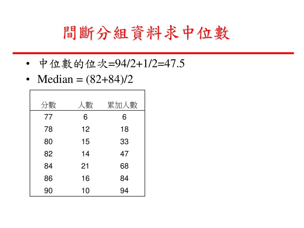
41 間斷性分組資料求中位數 間斷性分組資料求中位數的步驟： 將資料由小至大排序。 計算累加次數。 決定中位數所在的位次n/2+1/2。
如果中位數的位次剛好在組內，則取該組的數值x為中位數。如果位次落在兩組中間，則取兩組的平均值。

42 間斷分組資料求中位數 中位數的位次=94/2+1/2=47.5 Median = 82

43 間斷分組資料求中位數 中位數的位次=94/2+1/2=47.5 Median = (82+84)/2 分數 人數 累加人數 77 6 78
12 18 80 15 33 82 14 47 84 21 68 86 16 90 10 94

44 連續性分組資料中位數的推估 連續分組資料求中位數的步驟： 計算累加次數。 根據中位數所在的位次n/2，找出中位數所在的組別。
以下列公式求出中位數：

45 連續性分組資料中位數的推估

46 連續性分組資料中位數的推估 (1) 先將各組次數加總求出總次數，再用n/2的公式找到中位數的

47 連續性分組資料中位數的推估 (2)如果中位數的位次n/2介於Fi-1與Fi之間。 (3) 用C= Bi-Bi-1求得組距C 則中位數=

48 從第n/2個觀察值到本組的下界之間共有幾個觀察值
連續性分組資料中位數的推估 這個公式看起來有點複雜，其實很好理解。我們已知第n/2的數值落於該組中，我們想要找出最接近第n/2的位置的一個推估數值。 Fi-1 n/2 組距為C，組次數為f，C/f可以看成每個觀察值之間的單位距離 從第n/2個觀察值到本組的下界之間共有幾個觀察值

49 分組資料中位數的推估 請找出台灣地區成年人每週工時的中位數。

50 分組資料中位數的推估 步驟一：先算出累積次數 步驟二：找出中位數所在的組（n/2)。 n/2=1786/2=893

51 分組資料中位數的推估 步驟三：將組界調整成為不間斷 步驟四：套入公式求組中位數：
Median = (1786/2 – 291) * ( )/1001 = 46.51

52 中位數的特性 各觀察值與中位數差異的絕對值總和為最小。令α為任意數，則： 別忘了：

53 中位數的特性 Ordinal data較合適用中位數，而不適宜算平均值。 中位數不受觀察值之間的距離的影響。
中位數不受outlier 的影響。 數列一：8, 9, 10, 11, 12 數列二：0, 9, 10, 11, 1000

54 中位數的特性 若資料的分佈呈對稱分配 則中位數 = 平均值 若資料的分佈不對稱 中位數 中位數 平均值 平均值

55 中位數的特性 由於平均值易受偏離值的影響，當資料呈現偏峰分配時，計算中位數比平均值可能更具有代表性。

56 分位數 中位數又稱為二分位數，即將數字資料由小至大排序後，切成二部分。大於及小於中位數者剛好各佔所有數字資料的一半。
除了將資料作半切割外，我們也可以將資料切成四等分、十等分、或一百等分。 四分位數(Quartiles): Q1, Q2, Q3 十分位數(Deciles): D1, D2, D3, … 百分位數(Percentiles): P1, P2, P3, …

57 百分位數 Q1 = P25 Q3 =P75 Me = Q2=D5 =P50 n小於10，不求十分位數，n<100，不求百分位數。

58 百分位數 X1 X2 X3 Xp Xn p% (100-p)% Suppose the observations x1,x2,…xn have been arranged in ascending order. The pth percentile is the value xp such that p% of the observations are less than or equal to xp and (100-p)% of the observations are greater than or equal to xp. Xp為第p個百分位數，則「小於XP的觀察值佔所有觀察值的p%」。

59 未分組資料求百分位數 X1 X2 X3 Xp Xn Arrange the n observations in ascending order. 先將資料由小之大排序。 Calculate the index i = (p × n)/100, where p is the percentile of interest and n is the sample size.以p為所求之百分位，n為樣本數，計算出百分位數的位置i。 If i is an integer, the pth percentile is the arithmetic average of the values having ranks i and (i + 1). If i is not an integer, the next integer value greater than i denotes the rank of the value that is the pth percentile.

60 未分組資料求百分位數 X1 X2 X3 Xp Xn 1 p 100 整數，則p分位數= 第i與第(i+1)個觀察值的平均值
在一百個中間的第p個，相當於在n中間的第幾個？ i 非整數，則p分位數= i下一個觀察值

61 例題：求下列數列的70th 80th percentiles
重組： i =(70 ×15)/100 = 10.5 (not an integer) 第11個觀察值為70th percentile (70分位數）

62 例題：求下列數列的70th 80th percentiles
i =(80 ×15)/100 = 12 (an integer) 第12個觀察值為51，第13th觀察值為55 所以80 分位數 = (51+55)/2=53

63 分組資料求百分位數 有些統計學家認為分組資料應該用interpolating的方法來求 p 分位數： B=組下界
Fi-1=小於該組的各組次數和 f = 該組次數 C = 組距

64 四分位數(Quartiles) Q1 :25百分位數(25th percentile)又稱之為下四分位(lower quartile)或第一個四分位數(first quartile)，25%的觀察值在此數之下，75%的觀察值在此數之上。 Q3 : 75百分位數(75th percentile)又稱之為上四分位(upper quartile)或第三個四分位數(third quartile)，75%的觀察值在此數之下，25%的觀察值在此數之上。

65 眾數Mode The mode of a set of observations is the value that occurs with the greatest frequency. The mode is not necessarily unique. 未分組或列舉式資料：找出出現最多次數的觀察值，即為眾數Mo。

66 分組資料求眾數Mode 先在次數表中找出次數最多的那一組，稱為「眾數組」。 若取眾數組的組中點為眾數，則稱為「粗眾數」
Bimodal分配：如果一次數分配中出現兩個眾數。

67 分組資料求眾數Mode- King插補法 King差補法 眾數組 f-1 f+1 Mo B

68 分組資料求眾數Mode- King插補法 King差補法 組距 眾數組 組下界 前一組次數 後一組次數

69 分組資料求眾數Mode- King插補法 眾數組 當f-1>f+1時，眾數較靠近「組中點」的左方 f-1 f+1

70 分組資料求眾數Mode- King插補法 當f-1<f+1時，眾數較靠近「組中點」的右方 f-1 f+1

71 分組資料求眾數Mode- Czuber插補法

72 分組資料求眾數Mode- Czuber插補法

73 分組資料求眾數Mode- Pearson 經驗法

74 例題：用三種方法求眾數 粗眾數 = 45.5 King’s Mo = 40.5 +251/(172+251) ×10 = 46.43
粗眾數 = 45.5 King’s Mo = /( ) ×10 = 46.43 Czuber: ( ) ×10/[( )+( )]= 45.75 Pearson: Mo=48.38 –3( ) = 42.77

75 Common Shapes of Distributions
A distribution is said to be symmetric if the left half of the graph of the distribution is the mirror image of the right half. A distribution is said to be skewed if it is not symmetric. A distribution is skewed to the right if the right-hand tail of the distribution is longer than the left tail and most of the observations are concentrated in the left side f the distribution.

76 Common Shapes of Distributions
When a distribution is unimodal(單峰） and symmetric（對稱） like the bell-shaped normal distribution, the mean median, and the mode all coincide. 單峰對稱： Mean = Median =Mode 相對次數 Mean Median Mode

77 Common Shapes of Distributions
If the distribution is skewed to the right, the following relationships hold among the mean, median, and mode: 右偏分配（skewed to the right)： Mean > Median >Mode 相對次數 Mode Mean Median

78 Common Shapes of Distributions
If the distribution is skewed to the left, the following relationships hold among the mean, median, and mode: 左偏分配（skewed to the left)： Mean < Median <Mode 相對次數 Mode Median mean

79 Measures of Dispersion 分散量數、離差量數、差異量數
Summary statistics that measure the amount of variation in a data set are called measures of dispersion. 測量群體中各個觀察值之差異或離中程度的表徵數，即為離差量數。 離差小，表示各數值間的差異小，平均數較能代表群體中的各個數值，離差大，表各數值之間的變動很大，較為分散。 EX) 在財務管理的問題中，投資的風險即是以報酬的離差程度來衡量。

80 Range全距 The range of a set of observations is the difference between the largest value and the smallest value. 未分組資料 R = Xmax – Xmin(最大觀察值-最小值） 分組資料 R = Umax – Lmin(最大組之上界 –最小組之下界）

81 圖 資料的分散情形

82 Interquartile Range四分位距
IQR = Q3 – Q1 Semi-interquartile Range四分位差 QD = (Q3 – Q1) /2 ,即IQR的一半為四分位差。 Q3 - Md = Md – Q1 QD = Q3 - Md=Md - Q1 Md Q1 Q3 IQR

83 Deviation from the mean平均差
之前說平均值為所有觀察值的重力中心點，意旨高於此點的「正」平均差剛好等於低於此點的「負」平均差，如果將所有平均差加總，則： 由於平均差的和永遠等於零，因此無法用平均差來衡量資料分散的程度。

84 Mean Absolute Deviation 平均絕對差
為解決平均差正負相削的情形，可用「平均絕對差」( mean absolute deviation, M.A.D.) 來表示資料分散的平均情形；

85 Mean Absolute Deviation 平均絕對差
分組資料算M.A.D.: mi為組中點，fi為組次數 平均絕對差的缺點是，絕對值符號在數學運算上十分不便。

86 Population Variance σ2 Population Standard Deviation σ
一個衡量資料離散程度的常用指標為： 母體變異數 母體標準差

87 Sample Variance s2 Sample Standard Deviation s
樣本變異數 Degree of freedom 樣本標準差

88 Sample Variance s2 Sample Standard Deviation s
樣本變異數的簡易運算公式：

89 例題：求下列數列的標準差 樣本變異數與標準差

90 例題：求下列數列的標準差 步驟一： 先求平均數 步驟二：計算 平均數

91 例題：求下列數列的標準差 步驟三： 計算 = 20/(9-1) = 2.5

92 另解：求下列數列的標準差

93 分組資料求變異數及標準差

94 例題：求下列分組資料之變異數及標準差

95 例題：求下列分組資料之變異數及標準差 步驟一：先求出算數平均數

96 例題：求下列分組資料之變異數及標準差

97 另解：求下列分組資料之變異數及標準差

98 The Five-Number Summary
Minimum Q1 Md Q3 Maximum

99 Box Plot（箱型圖） Max Q3 Median IQR Q1 Min

100 Box Plot（箱型圖）

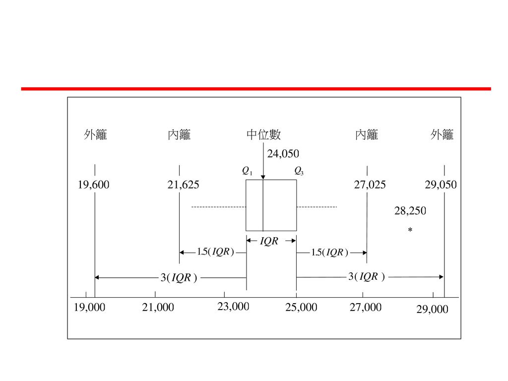
101 Box Plot（箱型圖） Extreme Outliers Q3 Median Q1 Outer fence
Extremes: Cases with values more than 3 box lengths from the upper or lower edge of the box. Inner fence Q3 IQR Median Q1 Cases with values between 1.5 and 3 box lengths from the upper or lower edge of the box. The box length is the IRQ. 1.5 IQR Inner fence 3 IQR Outliers Outer fence

102

103 男女生平均工時的敘述性統計 男性 女性 Statistics Statistics V46 V46 N Valid 1010 N Valid
741 Missing Missing Mean 49.06 Mean 47.92 Median 48.00 Median 48.00 Mode 48 Mode 48 Std. Deviation 13.12 Std. Deviation 13.16 Variance 172.10 Variance 173.18 Range 83 Range 88 Minimum 7 Minimum 2 Maximum 90 Maximum 90 Percentiles 25 44.00 Percentiles 25 44.00 50 48.00 50 48.00 75 56.00 75 50.00 男性 女性

104 outlier extreme

105 變異數與標準差之性質 S2≧0, 只有在所有觀察值皆相同時，等號才會成立。

106 變異數與標準差之性質 一群資料分成N1, N2, …Nk等k部分，各部分的相對平均數及變異數分別為μ1,σ12, μ2,σ22… μk,σk2 N1 N2 Nk μ1 …… μk μ2 σ12 σk2 σ22

107 變異數與標準差之性質 平均數： N1 N2 Nk μ1 …… μk μ2 σ12 σk2 σ22 各組平均數的加權平均數

108 變異數與標準差之性質 變異數： 觀察值與該組平均數之差 該組平均數與整體平均數之差 觀察值與平均數之差為零

109 變異數與標準差之性質 例題：已知社會系全體同學有以下的統計量： 男生40人,學期平均成績83分,標準差4分
女生200人，平均成績85分，標準差5分 請問全班的平均成績為何？標準差為何？

110 變異數與標準差之性質 N男=40人,μ男=83分, σ男=4分 N女=200人,μ女=85分, σ女=5分 全班平均分數：

111 變異數與標準差之性質 N男=40人,μ男=83分, σ男=4分 N女=200人,μ女=85分, σ女=5分 全班分數變異數：

112 Approximating a continuous distribution
觀念 取100人的樣本並紀錄其完成工作的時間如下：

113 Approximating a continuous distribution
觀念 以直方圖來表達：

114 Approximating a continuous distribution
觀念 將樣本擴大至1,000

115 Approximating a continuous distribution
觀念 將樣本擴大至10,000

116 Approximating a continuous distribution
觀念 將樣本擴大至100,000，隨著樣本數的增加，每一個變量之間的間隔愈小，曲線愈趨於平滑。 這個曲線可以被視為是根據母體（試驗重複很多次）的相對次數分配所畫出來的直方圖。 Density curve 密度曲線

117

118 以上累加相對次數

119 以下累加相對次數

120 Density Function 觀念 所有的“相對次數”的和為? 我們可以令曲線底下的面積和為1。 介於任意兩 x 值之間的機率。

121 Chebyshëv’s Theorem 徹比雪夫定理
Let c be any number greater than 1. For any sample or population of data, the proportion of observations that lie fewer than c standard deviations from the mean is at least (1 － 1 /c2). 無論資料為何種分配，令 c為任意大於1的常數，若一母體(或樣本）的平均數及標準差分別為μ及σ，則介於(μ－cσ, μ＋cσ)內之觀察值至少為(1 － 1 /c2)。

122 Chebyshëv’s Theorem 徹比雪夫定理
μ μ-cσ μ+cσ 當c=2時，至少75% (1-1/4)的觀察值落在平均數左右兩個標準差的範圍內。 當c=3時，至少89% (1-1/9)的觀察值落在平均數左右三個標準差的範圍內。 當c=4時，至少93% (1-1/16)的觀察值落在平均數左右四個標準差的範圍內。

123 The Empirical Rule 經驗法則
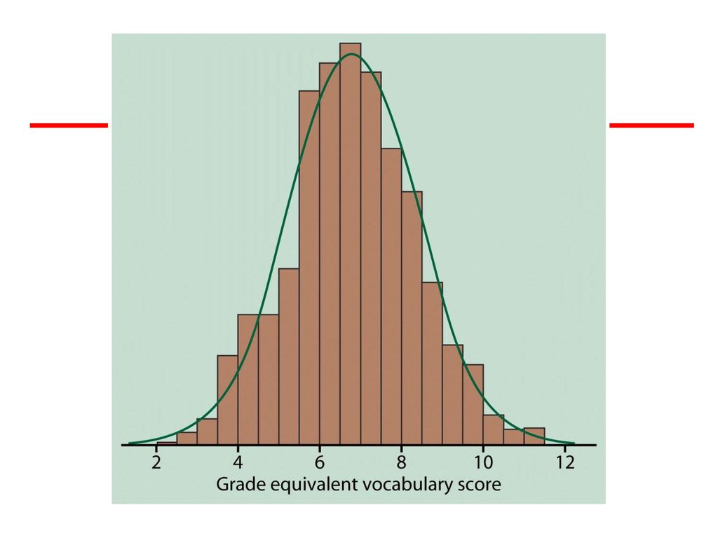
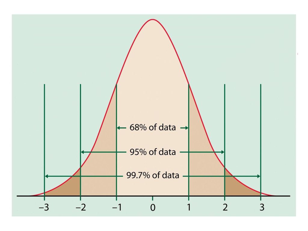
Chebyshëv’s Theorem是一個較保守的估計，如果我們知道確切的分佈，則能更精準的估算出落於某範圍的機率。 When the distribution of a population or sample of data is approximately bell shaped, approximately 68% of the values will fall within 1 standard deviation of the mean, approximately 95% of the values will fall within 2 standard deviations of the mean, and approximately 99.7% of the values will fall within 3 standard deviations of the mean.

124 The Empirical Rule 經驗法則
若資料呈現鐘形分配，則：

125

126 The Empirical Rule 經驗法則
若資料呈現鐘形分配，則： μ 68% μ-σ μ+σ 95% μ-2σ μ+2σ 99% μ+3σ μ-3σ

127 The Empirical Rule 經驗法則
Consider a bell-shaped distribution approximately ______ percentage of the values lies between μ-2σand μ+σ. 68% ÷2= 34% 95% ÷2= 47.5% μ 68% μ-σ 95% μ-2σ μ+σ μ+2σ

128 Coefficient of Variation 變異係數
The coefficient of variation, also called the relative standard deviation, expresses the standard deviation as a percentage of the mean. The CV allows us to consider the dispersion as a proportion of the mean, that is, the dispersion in proportion to the average magnitude of the data.

129 Coefficient of Variation 變異係數
B股票過去一年的平均價格為$50，標準差為$4。 請問哪一支股票的價格波動較厲害？ A股票的CV = 5/100 =5% B股票的CV=4/50 = 8%