Differential Equations (DE)

Presentation on theme: "Differential Equations (DE)"— Presentation transcript:

1 Differential Equations (DE)
工程數學--微分方程 Differential Equations (DE) 授課者：丁建均 教學網頁： (請上課前來這個網站將講義印好) 歡迎大家來修課！

2 授課者：丁建均 Office： 明達館723室, TEL： 33669652 Office hour： 週一至週五的下午皆可來找我
個人網頁：                上課時間： 星期三 第 3, 4 節 (AM 10:20~12:10)   星期五 第 2 節 (AM 9:10~10:00) 上課地點： 電二143 課本： "Differential Equations-with Boundary-Value Problem", 8th edition, Dennis G. Zill and Michael R. Cullen 評分方式：四次作業二次小考 15%,   期中考 42.5%,  期末考 42.5%    

3 注意事項： 請上課前，來這個網頁，將上課資料印好。 (2) 請各位同學踴躍出席 。 (3) 作業不可以抄襲。作業若寫錯但有用心寫仍可以有40%~90% 的分數，但抄襲或借人抄襲不給分。 (4) 我週一至週五下午都在辦公室，有什麼問題 ，歡迎同學們來找我

4 上課日期 Week Number Date (Wednesday, Friday) Remark 1. 9/16中秋節 2. 3. 4.
9/14 9/16中秋節  2. 9/21, 9/23 3. 9/28, 9/30 4. 10/5, 10/7 5. 10/12, 10/14 6. 10/19, 10/21 7. 10/26, 10/28  10/28 小考 8. 11/2, 11/4 9. 11/9: Midterm; (Chaps.1-5), 11/11  範圍： (Chaps.1-5) 10. 11/16, 11/18 11. 11/23, 11/25 12. 11/30, 12/2 13. 12/7, 12/9 14. 12/14  12/16 小考 15. 12/21, 12/23 16. 12/28, 12/30 17. 1/4, 1/6 18. 1/11 Finals  範圍： (Chaps. 6, 7, 11, 12, 14)

5 課程大綱 Introduction (Chap. 1) 解法 (Chap. 2) First Order DE 應用 (Chap. 3)
Higher Order DE 應用 (Chap. 5) 多項式解法 (Chap. 6) Partial DE (Chap. 12) Laplace Transform (Chap. 7) Transforms Fourier Series (Chap. 11) Fourier Transform (Chap. 14)

6 Chapter 1 Introduction to Differential Equations
1.1 Definitions and Terminology (術語) Differential Equation (DE): any equation containing derivation (page 2, definition 1.1) x: independent variable 自變數 y(x): dependent variable 應變數

7 Note: In the text book, f(x) is often simplified as f
notations of differentiation , , , , ………. Leibniz notation , , , , ………. prime notation , , , , ………. dot notation , , , , ………. subscript notation

8 (2) Ordinary Differential Equation (ODE):
differentiation with respect to one independent variable (3) Partial Differential Equation (PDE): differentiation with respect to two or more independent variables

9 (4) Order of a Differentiation Equation: the order of the highest derivative in the equation
7th order 2nd order

10 (5) Linear Differentiation Equation:
All of the coefficient terms am(x) m = 1, 2, …, n are independent of y. Property of linear differentiation equations: If and y3 = by1 + cy2, then (if g(x) is treated as the input and y(x) is the output)

11 (6) Non-Linear Differentiation Equation

12 (7) Explicit Solution (page 6)
The solution is expressed as y = (x) (8) Implicit Solution (page 7) Example: , Solution: (implicit solution) or (explicit solution)

13 1.2 Initial Value Problem (IVP)
A differentiation equation always has more than one solution. for , y = x, y = x+1 , y = x+2 … are all the solutions of the above differentiation equation. General form of the solution: y = x+ c, where c is any constant. The initial value (未必在 x = 0) is helpful for obtain the unique solution. and y(0) = y = x+2 and y(2) = y = x+1.5

14 The kth order differential equation usually requires k initial conditions (or k boundary conditions) to obtain the unique solution. solution: y = x2/2 + bx + c, b and c can be any constant y(1) = 2 and y(2) = 3 y(0) = 1 and y'(0) =5 y(0) = 1 and y'(3) =2 For the kth order differential equation, the initial conditions can be 0th ~ (k–1)th derivatives at some points. (boundary conditions，在不同點) (initial conditions ，在相同點) (boundary conditions，在不同點)

15 1.3 Differential Equations as Mathematical Model
Physical meaning of differentiation: the variation at certain time or certain place Example 1: x(t): location, v(t): velocity, a(t): acceleration F: force, β: coefficient of friction, m: mass

16 Example 2: 人口隨著時間而增加的模型
A: population 人口增加量和人口呈正比

17 Example 3: 開水溫度隨著時間會變冷的模型
T: 熱開水溫度, Tm: 環境溫度 t: 時間

18 大一微積分所學的： 例如： 的解 問題： (1) 若等號兩邊都出現 dependent variable (如 pages 16, 17 的例子) (2) 若order of DE 大於 1 該如何解？

19 DE Review dependent variable and independent variable PDE and ODE
Order of DE linear DE and nonlinear DE explicit solution and implicit solution initial value; boundary value IVP

20 Chapter 2 First Order Differential Equation
2-1 Solution Curves without a Solution Instead of using analytic methods, the DE can be solved by graphs (圖解) slopes and the field directions: y-axis the slope is f(x0, y0) (x0, y0) x-axis

21 Example dy/dx = 0.2xy From： Fig (a) in “Differential Equations-with Boundary-Value Problem”, 8th ed., Dennis G. Zill and Michael R. Cullen.

22 Example 2 dy/dx = sin(y), y(0) = –3/2
With initial conditions, one curve can be obtained From： Fig in “Differential Equations-with Boundary-Value Problem”, 8th ed., Dennis G. Zill and Michael R. Cullen.

23 Advantage: It can solve some 1st order DEs that cannot be solved by mathematics. Disadvantage: It can only be used for the case of the 1st order DE. It requires a lot of time

24 Section 2-6 A Numerical Method
Another way to solve the DE without analytic methods independent variable x x0, x1, x2, ………… Find the solution of Since approximation sampling(取樣) 前一點的值 取樣間格

25 Example: dy(x)/dx = 0.2xy y(xn+1) = y(xn) + 0.2xn y(xn )*(xn+1 –xn). dy/dx = sin(x) y(xn+1) = y(xn) + sin(xn)*(xn+1 –xn). 後頁為 dy/dx = sin(x), y(0) = –1, (a) xn+1 –xn = 0.01, (b) xn+1 –xn = 0.1, (c) xn+1 –xn = 1, (d) xn+1 –xn = 0.1, dy/dx = 10sin(10x) 的例子 Constraint for obtaining accurate results: (1) small sampling interval (2) small variation of f(x, y)

26 (a) (b) (c) (d)

27 Advantages -- It can solve some 1st order DEs that cannot be solved by mathematics. -- can be used for solving a complicated DE (not constrained for the 1st order case) -- suitable for computer simulation Disadvantages -- numerical error (數值方法的課程對此有詳細探討)

28 Exercises for Practicing
(not homework, but are encouraged to practice) 1-1: 1, 13, 19, 23, 33 1-2: 3, 13, 21, 33 1-3: 2, 7, 28 2-1: 1, 13, 20, 25, 33 2-6: 1, 3

29 附錄一 Methods of Solving the First Order Differential Equation
graphic method direct integration numerical method separable variable analytic method method for linear equation method for exact equation homogeneous equation method Bernoulli’s equation method method for Ax + By + c series solution Laplace transform matrix solution Fourier series Fourier cosine series transform Fourier sine series Fourier transform

30 Simplest method for solving the 1st order DE: Direct Integration
dy(x)/dx = f(x) where

31 附錄二 Table of Integration
1/x ln|x| + c cos(x) sin(x) + c sin(x) –cos(x) + c tan(x) –ln|cos(x)| + c cot(x) ln|sin(x)| + c ax ax/ln(a) + c x eax x2 eax

32 Others about Integration
例： (2) 算完 integration 之後不要忘了加 constant c (3) If then c1 is also some constant

33 2-2 Separable Variables 2-2-1 方法的限制條件
方法的限制條件 1st order DE 的一般型態: dy(x)/dx = f(x, y) [Definition 2.2.1] (text page 46) If dy(x)/dx = f(x, y) and f(x, y) can be separate as f(x, y) = g(x)h(y) i.e., dy(x)/dx = g(x)h(y) then the 1st order DE is separable (or have separable variable).

34 條件： dy(x)/dx = g(x)h(y)

35 2-2-2 解法 If , then Step 1 where p(y) = 1/h(y) 分離變數 Step 2 where 個別積分
解法 If , then Step 1 where p(y) = 1/h(y) Step 2 where 分離變數 個別積分 Extra Step: (a) Initial conditions (b) Check the singular solution (i.e., the constant solution)

36 Extra Step (b) Check the singular solution (常數解):
Suppose that y is a constant r solution for r See whether the solution is a special case of the general solution.

37 2-2-3 Examples Example 1 (text page 47) (1 + x) dy – y dx = 0
Extra Step (b) check the singular solution Step 1 set y = r , 0 = r/(1+x) r = 0, y = 0 Step 2 (a special case of the general solution)

38 Example 練習小技巧 遮住解答和筆記，自行重新算一次 (任何和解題有關的提示皆遮住) Exercise 練習小技巧 初學者，先針對有解答的題目作練習 累積一定的程度和經驗後，再多練習沒有解答的題目 將題目依類型分類，多綀習解題正確率較低的題型 動筆自己算，就對了

39 Example 2 (with initial condition and implicit solution, text page 48)
, y(4) = –3 Extra Step (b) check the singular solution Step 1 Step 2 Extra Step (a) (implicit solution) invalid valid (explicit solution)

40 Example 3 (with singular solution, text page 48)
Extra Step (b) check the singular solution Step 1 set y = r , 0 = r2 – 4 r = 2, y = 2 Step 2 or y = 2

41 Example 4 (text page 49) 自修 注意如何計算 ,

42 Example in the top of page 50
, y(0) = 0 Extra Step (b) Check the singular solution Step 1 Step 2 Extra Step (a) Solution: or

43 補充：其實， 這一題還有更多的解 , y(0) = 0 solutions: (1) (2) (3) b  0  a

44 2-2-4 IVP 是否有唯一解？ 這個問題有唯一解的條件：(Theorem 1.2.1, text page 16)
如果 f(x, y), 　　　　　 在 x = x0, y = y0 的地方為 continuous 則必定存在一個 h，使得 IVP 在 x0−h < x < x0 +h 的區間當中有唯一解

45 2-2-5 Solutions Defined by Integral
(1) (2) If dy/dx = g(x) and y(x0) = y0, then 積分 (integral, antiderivative) 難以計算的 function， 被稱作是 nonelementary 如 , 此時，solution 就可以寫成 的型態

46 Example 5 (text page 50) Solution 或者可以表示成 complementary error function

47  error function (useful in probability)
 complementary error function 用 t 取代 x 以做區別 See text page 59 in Section 2.3

48 2-2-6 本節要注意的地方 (1) 複習並背熟幾個重要公式的積分 (2) 別忘了加 c 並且熟悉什麼情況下 c 可以合併和簡化
本節要注意的地方 (1) 複習並背熟幾個重要公式的積分 (2) 別忘了加 c 並且熟悉什麼情況下 c 可以合併和簡化 (3) 若時間允許，可以算一算 singular solution (4) 多練習，加快運算速度

49 附錄三 微分方程查詢 http://integrals.wolfram.com/index.jsp 輸入數學式，就可以查到積分的結果 範例：
附錄三 微分方程查詢 輸入數學式，就可以查到積分的結果 範例： (a) 先到integrals.wolfram.com/index.jsp 這個網站 (b) 在右方的空格中輸入數學式，例如 數學式

50 (c) 接著按 “Compute Online with Mathematica” 就可以算出積分的結果

51 (d) 有時，對於一些較複雜的數學式，下方還有連結，點進去就可以看到相關的解說
.,,,,,,,,l,,,,,,,l,,,lll,,,,k,l 連結

52 其他有用的網站 對微分方程的定理和名詞作介紹的百科網站 眾多數學式的 mathematical table (不限於微分方程) 眾多數學式的 mathematical table，包括 convolution, Fourier transform, Laplace transform, Z transform 軟體當中， Maple, Mathematica, Matlab 皆有微積分結果查詢有功能

53 2-3 Linear Equations 2-3-1 方法的適用條件 “friendly” form of DEs
方法的適用條件 [Definition 2.3.1] The first-order DE is a linear equation if it has the following form: g(x) = 0: homogeneous g(x)  0: nonhomogeneous

54 Standard form: 許多自然界的現象，皆可以表示成 linear first order DE

55 2-3-2 解法的推導 子問題 1 子問題 2 Find the general solution yc(x)
解法的推導 子問題 1 子問題 2 Find the general solution yc(x) (homogeneous solution) Find any solution yp(x) (particular solution) Solution of the DE

56  yc + yp is a solution of the linear first order DE, since
Any solution of the linear first order DE should have the form yc + yp . The proof is as follows. If y is a solution of the DE, then Thus, y − yp should be the solution of y should have the form of y = yc + yp

57 Solving the homogeneous solution yc(x) (子問題一）
separable variable Set , then

58 Solving the particular solution yp(x) (子問題二）
Set yp(x) = u(x) y1(x) (猜測 particular solution 和 homogeneous solution 有類似的關係) equal to zero

59 solution of the linear 1st order DE:
where c is any constant : integrating factor

60 2-3-3 解法 (Step 1) Obtain the standard form and find P(x)
解法 (Step 1) Obtain the standard form and find P(x) (Step 2) Calculate (Step 3a) The standard form of the linear 1st order DE can be rewritten as: (Step 3b) Integrate both sides of the above equation remember it or remember it, skip Step 3a (Extra Step) (a) Initial value (c) Check the Singular Point

61 Singular points: the locations where a1(x) = 0
i.e., P(x)   More generally, even if a1(x)  0 but P(x)   or f(x)  , then the location is also treated as a singular point. (a) Sometimes, the solution may not be defined on the interval including the singular points. (such as Example 4) (b) Sometimes the solution can be defined at the singular points, such as Example 3

62 More generally, even if a1(x)  0 but P(x)   or f(x)  , then the location is also treated as a singular point. Exercise 33

63 例子 Example 2 (text page 56) Extra Step (c) Step 1 check the singular point Step 2 為何在此時可以將 –3x+c 簡化成 –3x? Step 3 或著，跳過 Step 3，直接代公式 Step 4

64 Example 3 (text page 57) Extra Step (c) check the singular point Step 1 x = 0 Step 2 思考： x < 0 的情形 若只考慮 x > 0 的情形, Step 3 Step 4 x 的範圍: (0, )

65 Example 4 (text page 58) Extra Step (c) check the singular point defined for x  (–, –3), (–3, 3), or (3, ) not includes the points of x = –3, 3

66 Example 6 (text, page 59) check the singular point 0  x  1 x > 1 要求 y(x) 在 x = 1 的地方為 continuous from initial condition

67 2-3-5 名詞和定義 (1) transient term, stable term
名詞和定義 (1) transient term, stable term Example 5 (text page 58) 的解為 : transient term 當 x 很大時會消失 x 1: stable term y x1 x-axis

68 (2) piecewise continuous
A function g(x) is piecewise continuous in the region of [x1, x2] if g'(x) exists for any x  [x1, x2]. In Example 6, f(x) is piecewise continuous in the region of [0, 1) or (1, ) (3) Integral (積分) 有時又被稱作 antiderivative (4) error function complementary error function

69 (5) sine integral function
Fresnel integral function (6) f(x) 常被稱作 input 或 deriving function Solution y(x) 常被稱作 output 或 response

70 2-3-6 小技巧 When is not easy to calculate: Try to calculate Example:
小技巧 When is not easy to calculate: Try to calculate Example: (not linear, not separable) (linear) (implicit solution)

71 2-3-7 本節要注意的地方 (1) 要先將 linear 1st order DE 變成 standard form
本節要注意的地方 (1) 要先將 linear 1st order DE 變成 standard form (2) 別忘了 singular point 注意：singular point 和 Section 2-2 提到的 singular solution 不同 (3) 記熟公式 或 (4) 計算時， 的常數項可以忽略

72 太多公式和算法，怎麼辦？ 最上策： realize + remember it 上策： realize it 中策： remember it 下策： read it without realization and remembrance 最下策： rest z…..z..…z……

73 Chapter 3 Modeling with First-Order Differential Equations
應用題 Convert a question into a 1st order DE. 將問題翻譯成數學式 (2) Many of the DEs can be solved by Separable variable method or Linear equation method (with integration table remembrance)

74 3-1 Linear Models Growth and Decay (Examples 1~3)
Change the Temperature (Example 4) Mixtures (Example 5) Series Circuit (Example 6) 可以用 Section 2-3 的方法來解

75 Example 1 (an example of growth and decay, text page 84)
Initial: A culture (培養皿) initially has P0 number of bacteria. The other initial condition: At t = 1 h, the number of bacteria is measured to be 3P0/2. 關鍵句: If the rate of growth is proportional to the number of bacteria A(t) presented at time t, Question: determine the time necessary for the number of bacteria to triple 翻譯  A(0) = P0 翻譯  A(1) = 3P0/2 翻譯  k is a constant 翻譯  find t such that A(t) = 3P0 這裡將課本的 P(t) 改成 A(t)

76 A(0) = P0, A(1) = 3P0/2 可以用 什麼方法解？ Extra Step (b)
check singular solution Step 1 Step 2 Extra Step (a) (1) c = P0 (2) k = ln(3/2) = 針對這一題的問題

77 課本用 linear (Section 2.3) 的方法來解 Example 1
思考：為什麼此時需要兩個 initial values 才可以算出唯一解？

78 Example 4 (an example of temperature change, text page 86)
Initial: When a cake is removed from an oven, its temperature is measured at 300 F. 翻譯  T(0) = 300 The other initial condition: Three minutes later its temperature is 200  F. 翻譯  T(3) = 200 question: Suppose that the room temperature is 70 F. How long will it take for the cake to cool off to 75 F? (註：這裡將課本的問題做一些修改) 翻譯  find t such that T(t) = 75. 另外，根據題意，了解這是一個物體溫度和周圍環境的溫度交互作用的問題，所以 T(t) 所對應的 DE 可以寫成 k is a constant

79 T(0) = 300 T(3) = 200 課本用 separable variable 的方法解 如何用 linear 的方法來解？

80 Example 5 (an example for mixture, text page 87)
Concentration: 2 lb/gal 300 gallons 3 gal/min 3 gal/min A: the amount of salt in the tank

81

82 LR series circuit From Kirchhoff’s second law

83 RC series circuit q: 電荷

84 How about an LRC series circuit?

85 Example 7 (text page 89) LR series circuit
 E(t): 12 volt,  inductance: 1/2 henry,  resistance: 10 ohms,  initial current: 0 這裡 + c1 可省略

86 Circuit problem for t is small and t 
For the LR circuit: L R transient stable For the RC circuit: R C transient stable

87 3-2 Nonlinear Models 3-2-1 Logistic Equation
可以用 separable variable 或其他的方法來解 Logistic Equation used for describing the growth of population The solution of a logistic equation is called the logistic function. Two stable conditions: and

88 Logistic curves for differential initial conditions

89 Solving the logistic equation
separable variable 註： (with initial condition P(0) = P0) logistic function

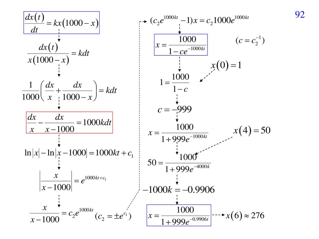
90 Example 1 (text page 97) There are 1000 students.
 Suppose a student carrying a flu virus returns to an isolate college campus of 1000 students.  If it is assumed that the rate at which the virus spreads is proportional not only to the number x of infected students but also to the number of students not infected, 翻譯  x(0) = 1 翻譯  k is a constant  determine the number of infected students after 6 days 翻譯  find x(6)  if it is further observed that after 4 days x(4) = 50

91 整個問題翻譯成 Initial: x(0) = 1, x(4) = 50 find x(6) 可以用separable variable 的方法

92

93 Logistic equation 的變形 (1) 人口有遷移的情形 (2) 遷出的人口和人口量呈正比 (3) 人口越多，遷入的人口越少 (4) Gompertz DE 飽合人口為 人口增加量，和 呈正比

94 3-2-2 化學反應的速度 A + B  C Use compounds A and B to for compound C
化學反應的速度 A + B  C Use compounds A and B to for compound C x(t): the amount of C To form a unit of C requires s1 units of A and s2 units of B a: the original amount of A b: the original amount of B The rate of generating C is proportional to the product of the amount of A and the amount of B See Example 2