1 時 頻 分 析 近 年 來 的 發 展時 頻 分 析 近 年 來 的 發 展 丁 建 均 國立台灣大學電信工程學研究所 Recent Development of Time-Frequency Analysis.

Presentation on theme: "1 時 頻 分 析 近 年 來 的 發 展時 頻 分 析 近 年 來 的 發 展 丁 建 均 國立台灣大學電信工程學研究所 Recent Development of Time-Frequency Analysis."— Presentation transcript:

1

2 1 時 頻 分 析 近 年 來 的 發 展時 頻 分 析 近 年 來 的 發 展 丁 建 均 國立台灣大學電信工程學研究所 Recent Development of Time-Frequency Analysis

3 2 一、什麼是時頻分析 (Time-Frequency Analysis) Fourier transform 不足的地方： Frequency Analysis: by Fourier transform (FT) 無法看出頻率隨著時間而改變的情形

4 3 x(t) = cos(440  t) when t < 0.5, x(t) = cos(660  t) when 0.5  t < 1, x(t) = cos(524  t) when t  1 The Fourier transform of x(t) Frequency Example 1

5 4 Short-Time Fourier Transform w(t): mask function 也稱作 windowed Fourier transform 或 time-dependent Fourier transform 例如：

6 5 Example: x(t) = cos(440  t) when t < 0.5, x(t) = cos(660  t) when 0.5  t < 1, x(t) = cos(524  t) when t  1 用 Gray level 來表示 X(t, f) 的 amplitude t–axis (Second) f -axis (Hertz)

7 6 瞬 時 頻 率 (Instantaneous Frequency) If then the instantaneous frequency is If the order of > 1, then instantaneous frequency varies with time

8 7 Example 2 t  [0, 3] 瞬 時 頻 率瞬 時 頻 率 (a) (b) 瞬 時 頻 率瞬 時 頻 率 t  [0, 3]

9 8 Fourier transform f (Hz)

10 9 Short-time Fourier transform

11 10 頻率會隨著時間而變化的例子： Frequency Modulation (FM) Signal Speech Music Others (Animal voice, Doppler effect, seismic waves, radar system, optics, rectangular function) In fact, in addition to sinusoid-like functions, the instantaneous frequencies of other functions will inevitably vary with time.

12 11 二、時頻分析的分類和發展歷史

13 12 時頻分析理論發展年表 AD 1785 The Laplace transform was invented AD 1812 The Fourier transform was invented AD 1822 The work of the Fourier transform was published AD 1910 The Haar Transform was proposed AD 1927 Heisenberg discovered the uncertainty principle AD 1929 The fractional Fourier transform was invented by Wiener AD 1932 The Wigner distribution function was proposed AD 1946 The short-time Fourier transform and the Gabor transform was proposed. (In the same year, the computer was invented) AD 1961 Slepian and Pollak found the prolate spheroidal wave function AD 1966 Cohen’s class distribution was invented

14 13 AD 1971 Moshinsky and Quesne proposed the linear canonical transform AD 1980 The fractional Fourier transform was re-invented by Namias AD 1981 Morlet proposed the wavelet transform AD 1982 The relations between the random process and the Wigner distribution function was found by Martin and Flandrin AD 1988 Mallat and Meyer proposed the multiresolution structure of the wavelet transform; In the same year, Daubechies proposed the compact support orthogonal wavelet AD 1989 The Choi-Williams distribution was proposed; In the same year, Mallat proposed the fast wavelet transform AD 1990 The cone-Shape distribution was proposed by Zhao, Atlas, and Marks AD 1993 Mallat and Zhang proposed the matching pursuit; In the same year, the rotation relation between the WDF and the fractional Fourier transform was found by Lohmann

15 14 AD 1994 The applications of the fractional Fourier transform in signal processing were found by Almeida, Ozaktas, Wolf, Lohmann, and Pei AD 1995 L. J. Stankovic, S. Stankovic, and Fakultet proposed the pseudo Wigner distribution AD 1996 Stockwell, Mansinha, and Lowe proposed the S transform AD 1998 N. E. Huang proposed the Hilbert-Huang transform AD 1999 Candes, Donoho, Antoine, Murenzi, and Vandergheynst proposed the directional wavelet transform AD 2000 The standard of JPEG 2000 was published by ISO AD 2002 Stankovic proposed the time frequency distribution with complex arguments AD 2003 Pinnegar and Mansinha proposed the general form of the S transform AD 2007 The Gabor-Wigner transform was proposed by Pei and Ding

16 15 時頻分析理論的五大家族 (1) Short-Time Fourier transform 家族 (2) Wigner distribution function 家族 (3) Wavelet transform 家族 (4) Time-Variant Basis Expansion 家族 (5) Hilbert-Huang transform 家族

17 16 時頻分析的大家族 (1) Short-time Fourier transform (STFT) (rec-STFT, Gabor, …) square spectrogram improve S transform (2) Wigner distribution function (WDF) combine Gabor-Wigner Transform improve windowed WDF improve Cohen’s Class Distribution (Choi-Williams, Cone-Shape, Page, Levin, Kirkwood, Born-Jordan, …) improve Pseudo L-Wigner Distribution (4) Time-Variant Basis Expansion Matching Pursuit Prolate Spheroidal Wave Function (5) Hilbert-Huang Transform (3) Wavelet transform Haar and Daubechies Coiflet, Morlet Directional Wavelet Transform ( 唯一跳脫 Fourier transform 的架構 ) Asymmetric STFT

18 17 (1) Short-Time Fourier Transform (2) Wigner Distribution Function

19 18 Simulations x(t) = cos(2  t) by WDF by short-time Fourier transform f-axis t-axis

20 19 (3) Wavelet Transform x 1,L [n] x 1,H [n] g[n] x[n]x[n] h[n]  2 x[n] 的低頻成份 x[n] 的高頻成份 lowpass filter highpass filter down sampling xL[n]xL[n] xH[n]xH[n] N-points L-points

21 20 例子： 2-point Haar wavelet g[n] = 1/2 for n = −1, 0 g[n] = 0 otherwise h[0] = 1/2, h[−1] = −1/2, h[n] = 0 otherwise n g[n] -3 -2 -1 0 1 2 3 ½ n h[n] -3 -2 -1 0 1 2 3 ½ -½ then ( 兩點平均 )( 兩點之差 )

22 21 x[m, n] g[n]g[n] h[n]h[n]  2 along n v 1,L [m, n] v 1,H [m, n] g[m]g[m] h[m]h[m] along m  2 x 1,L [m, n]  2 along m x 1,H1 [m, n] g[m]g[m] h[m]h[m] along m  2 x 1,H2 [m, n] x 1,H3 [m, n] 2-D 的情形 m 低頻, n 低頻 m 高頻, n 低頻 m 低頻, n 高頻 m 高頻, n 高頻 L-points M ×N n m

23 22 原影像 2-D DWT 的結果 x 1,L [m, n] x 1,H1 [m, n] x 1,H2 [m, n] x 1,H3 [m, n]

24 23 3 次 2-D DWT 的結果

25 24 三、時頻分析近年來的發展 (1) Problem about Computation Time (2) New Time-Frequency Analysis Tool Asymmetric short-time Fourier transform Hilbert-Huang transform Gabor-Wigner transform Directional Wavelet transform (3) New Applications Adaptive sampling theory Biology S transform Adaptive filter design

26 25 3-1 Problem about Computation Time (1) 對於許多信號的時頻分佈而言 和之間有高度的相關性 (2) 可預測瞬時頻率的位置 大部分信號瞬時頻率都偏低頻 且只要是由樂器或生物聲帶產生的信號，都會有 「倍頻」的現象 “Adaptive interval” and “interpolation”

27 26 Short-time Fourier transform of a music signal   = 1/44100 ( 總共有 44100  1.6077 sec + 1 = 70902 點

28 27 with adaptive output sampling intervals

29 28 時頻分析的大家族 (1) Short-time Fourier transform (STFT) (rec-STFT, Gabor, …) square spectrogram improve S transform (2) Wigner distribution function (WDF) combine Gabor-Wigner Transform improve windowed WDF improve Cohen’s Class Distribution (Choi-Williams, Cone-Shape, Page, Levin, Kirkwood, Born-Jordan, …) improve Pseudo L-Wigner Distribution (4) Time-Variant Basis Expansion Matching Pursuit Prolate Spheroidal Wave Function (5) Hilbert-Huang Transform (3) Wavelet transform Haar and Daubechies Coiflet, Morlet Directional Wavelet Transform ( 唯一跳脫 Fourier transform 的架構 ) Asymmetric STFT

30 29 3-2 Asymmetric Short-Time Fourier Transform Short-Time Fourier Transform 通常 w(t) 是左右對稱的 但是在某些應用 ( 例如地震波的偵測 ) 使用非對稱的 window 會有較好的效果

31 30 3-3 S Transform [Ref] R. G. Stockwell, L. Mansinha, and R. P. Lowe, “Localization of the complex spectrum: the S transform,” IEEE Trans. Signal Processing, vol. 44, no. 4, pp. 998–1001, Apr. 1996. 比較：原本的 short-time Fourier transform 當 w(t) = exp(  t 2 ) 時 f , window width  f , window width 

32 31 x(t) = cos(  t) when t < 10, x(t) = cos(3  t) when 10  t < 20, x(t) = cos(2  t) when t  20 Using the short-time Fourier transform

33 32 x(t) = cos(  t) when t < 10, x(t) = cos(3  t) when 10  t < 20, x(t) = cos(2  t) when t  20 Using the S transform

34 33 3-4 Gabor-Wigner Transform 如何同時達成 (1) high clarity (2) no cross-term 的目標？ by WDF by short-time Fourier transform f-axis t-axis cos(2  t)

35 34 Short-time Fourier transform Wigner [Ref] S. C. Pei and J. J. Ding, “Relations between Gabor transforms and fractional Fourier transforms and their applications for signal processing,” IEEE Trans. Signal Processing, vol. 55, no. 10, pp. 4839-4850, Oct. 2007.

36 35 3-5 Directional Wavelet Transform Wavelet transform 未必要沿著 x, y 軸來做  curvelet  contourlet  bandlet  shearlet  Fresnelet  wedgelet  brushlet

37 36  Bandlet 根據物體的紋理或邊界，來調整 wavelet transforms 的方向 Stephane Mallet and Gabriel Peyre, "A review of Bandlet methods for geometrical image representation," Numerical Algorithms, Apr. 2002.

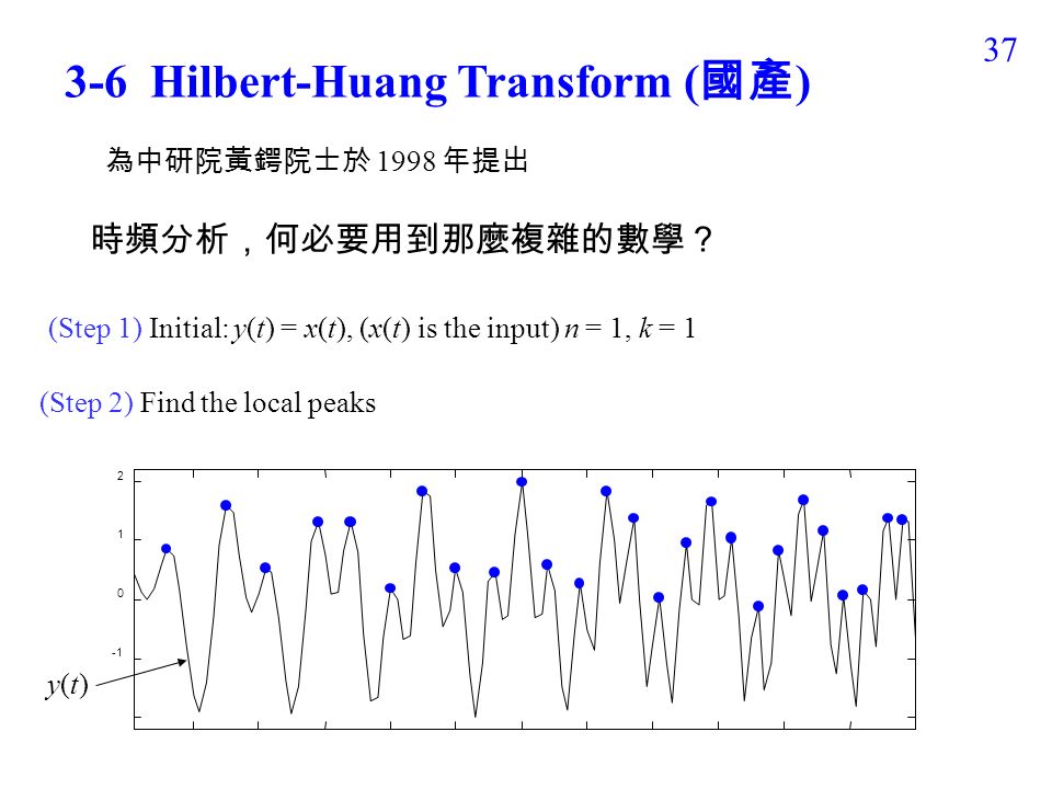
38 37 3-6 Hilbert-Huang Transform ( 國產 ) 時頻分析，何必要用到那麼複雜的數學？ (Step 2) Find the local peaks 0 1 2 y(t) (Step 1) Initial: y(t) = x(t), (x(t) is the input) n = 1, k = 1 為中研院黃鍔院士於 1998 年提出

39 38 (Step 3) Connect local peaks 0 1 2 IMF 1; iteration 0 通常使用 B-spline ，尤其是 cubic B-spline 來連接

40 39 (Step 4) Find the local dips (Step 5) Connect the local dips

41 40 (Step 6-1) Compute the mean (pink line) (Step 6-2) Compute the residue -1.5 -0.5 0 0.5 1 1.5

42 41 Step 7 Repeat Steps 1-6 to determine the intrinsic mode function (IMF) Step 8 Repeat Steps 1-7 to further determine x(t) Step 9 Determine the instantaneous frequency for each IMF (just calculating the number of zero-crossing during [t-1/2, t+1/2])

43 42 Example After Step 6

44 43 IMF1 IMF2 x0(t)x0(t) 趨勢

45 44 3-7 Application: Adaptive Sampling Nyquist rate:  t < 1/2B B: bandwidth

46 45 重要定理： Number of sampling points == Area of time frequency distribution

47 46 3-8 Application: Adaptive Filter Design Adaptive cutoff

48 47 3-9 Applications in Biology Data source: http://oalib.hlsresearch.com/Whales/index.htmlhttp://oalib.hlsresearch.com/Whales/index.html Whale voice

49 48 四、結 論 (1) 由於計算速度的大幅提升，使得使用「時頻分析」來取代「傅立葉轉 換」來做信號分析變得更加可行 (2) 時頻分析新理論和新應用的發展，有待大家共同努力 所有傅立葉轉換的應用 都將會是時頻分析的應用 http://djj.ee.ntu.edu.tw/TF.ppt 投影片下載網址：