統計學(Statistics) 其 目的 應用.

Presentation on theme: "統計學(Statistics) 其 目的 應用."— Presentation transcript:

1 統計學(Statistics) 其 目的 應用

2 應用 在 會計 財務 行銷 生產 經濟 如 例子

3 會計 財務 行銷 生產 經濟 風險測度 投資報酬 促銷成效 市場調查 品質管制 最適決策 期望效用 失業率 審計風險 審計抽樣 型Ⅰ風險
如 如 如 如 如 風險測度 投資報酬 促銷成效 市場調查 品質管制 最適決策 期望效用 失業率 審計風險 審計抽樣 應用 應用 應用 應用 應用 應用 應用 應用 應用 應用 型Ⅰ風險 統計抽樣 標準差 平均數 迴歸分析 統計抽樣 機率原理 貝氏定理 期望值 機率

4 目的 在 解釋 蒐集 整理 呈現 分析 資料（data）

5 測量尺度 資 料 測量值(measurements) 表1.1 元素(elements) 時間 屬性 橫斷面資料 時間數列資料 定量資料
參考例子 表1.1 資 料 乃是 測量值(measurements) 蒐集的實體稱為 種類依 元素(elements) 測量尺度 時間 有無限制細分 屬性 其中有興趣 的屬性稱為 分 為 分 為 分 為 橫斷面資料 時間數列資料 定量資料 定性資料 離散型資料 連續型資料 變數(variables) 可為 為 數值型態 數值型態 非數值型態

6 Variable: nominal scale elements
Ticker Symbol Price/earning ratio Gross Profit Margin Company Exchange Market Cap 36.7 DeWolfe Companies AMEX DWL 36.4 8.4 52.5 6.2 North Cost Energy OTC NCEB 59.3 14.6 44.8 41.1 Hansen Natural Corp. OTC HANS nominal scale elements Variable: Characteristic of interest for the elements

7 名目尺度(nominal scale): When the data for a variable consist of labels or names used to identify an attribute of the element . 順序尺度(ordinal scale): If the exhibit the properties of nominal data and the order or rank of the data is meaningful. 區間尺度(interval scale): If the data show the properties of ordinal data and the interval between values is expressed in terms of a fixed unit of measure. 比例尺度(ratio scale): If the data have all the properties of interval data and the ratio of two values is meaningful.

8 測量尺度 名目尺度 順序尺度 區間尺度 比例尺度 顏色 定性資料(Qualitive data) 數值、非數值皆可 定量資料
ex ex ex ex 服務品質︰ 傑出.好.不佳 學業成績 ５０，９０分 條件 : 必須包含零值 如 : 距離.高度.重量 顏色 定性資料(Qualitive data) 數值、非數值皆可 定量資料 (Qantitative variable) 算術運算對此有意義

9 定量資料 For purposes of statistical analysis , distinguishing… 時間序列資料
(time series data) 橫斷面資料 (cross-sectional data) Data collected over several time periods. Data collected at the same or approximately the same point in time. 例:圖一 例子

10 ex:時間序列資料 (圖一)

11 (statistical inference)
資 料 來源 統計推論 (statistical inference) 敘 述 統 計(descriptive statistics) 現存資料 統計研究 將資訊統計以讓人易瞭解的資料形式呈現 Experimental 工具 包含 Observational 新藥實驗 Tabular Numerical 例:餐廳以觀察研究調查顧客對食物、服務等滿意程度 Graphical

12 統計推論(statistical inference):
Statistics uses data from a sample(樣本) to make estimates and test hypotheses about the characteristics of a population(母體) through a process referred to as statistical inference. 利用樣本所得的資料對母體特性做評估與假設檢定 Ex : Norris電子公司的統計推論過程

13 The process of statistical inference for the NORRIS electronics example
1.Population consists of all bulbs manufactured with the new filament. Average lifetime is unknown. 2.A sample of 200bulbs is manufactured with the new filament. 4.The sample average is used to estimate the population average. 3.The sample data provide a sample average lifetime of 76 hours per bulb.

14 敘述統計 工具 包含 定性資料 定量資料

15 定性資料 表格 圖形 數值 單變數 兩變數 長條圖 圓餅圖 交叉表格 百分比次數分配表 次數分配表 相對次數分配表 例子 例子

16 次數分配(Frequency distribution)
A frequency distribution is a tabular summary of data showing the number (frequency) of items in each of several nonoverlapping classes. 設所購買的50瓶飲料中,各種飲料的出現次數: Soft Drink Frequency Coke Classic Diet Coke Dr. Pepper Pepsi-Cola Sprite total

17 Relative frequency And percent frequency distribution
Frequency of the class 公式:Relative frequency= n Soft Drink Coke Classic Diet Coke Dr. Pepper Pepsi-Cola Sprite total Relative frequency .38 .16 .10 .26 Percent frequency 38 16 10 26 1.00 100

18 長條圖(Bar Graph) Is a graphical device for depicting qualitative data summarized in a frequency, relative frequency, or percent frequency distribution.

19 圓餅圖(pie chart) 用來表示定性資料相對次數分配及百分比次數所對應的圖形

20 定量資料 表格 圖形 數值 點圖 直方圖 肩行圖 多邊形圖 莖葉圖 次數分配表 相對次數分配表 百分比次數分配表 累積次數分配表
單變數 兩變數 點圖 直方圖 肩行圖 多邊形圖 莖葉圖 次數分配表 相對次數分配表 百分比次數分配表 累積次數分配表 累積相對次數分配表 累積百分比次數分配表 交叉表格 兩變數 散佈圖

21 次數分配(Frequency distribution)
EX:表2.5(見課本P.31)為會計公司為20位客戶完成年終稽核所需的天數,為定量資料做次數分配,須先完成以下步驟: 1. Determine the number of nonoverlapping classes. (決定不相重疊的組別數目) 2. Determine the width of each class.(決定組寬) 3. Determine the class limits.(決定組界)

22 Number of classes(組數):
The goal is to use enough classes to show the variation in the data. Width of the classes(組寬): As the general guideline, we recommend that the width be the same for each class. . Largest data value – Small data value 公式: Number of classes

23 Class limits(組限): Class limits must be chosen so that each data item belongs to one and only one class. Class midpoint(組中點): In some applications, we want to know the midpoints of the classes in a frequency distribution for quantitative data.

24 frequency distribution for the audit time data
TABLE2.5 YEAR-END AUDIT TIMES (IN DAYS) frequency distribution for the audit time data audit time (days) 10-14 15-19 20-24 25-29 30-34 Frequency 4 8 5 2 1 組數:4 上組界:24 下組界:20 組寬: (33-12)/5=4.2 Total:

25 直方圖(histogram) 資料須先經過彙整(如:次數分配、百分比次數分配等) 可了解資料分布的形狀 (圖形請參照課本P.34)

26 點圖(dot plot) 最簡單的圖形彙總之ㄧ 比較兩個以上資料分布十分有用 圖形請參照課本P.33)

27 累積分配(cumulative distributions)
累積次數分配(cumulative frequency distributions) 累積相對次數分配(cumulative relative frequency distributions) 累積百分比次數分配(cumulative percent frequency distributions)

28 累積次數分配 (cumulative frequency distributions)
稽核時間 累積次數 累積相對次數 累積百分比次數 ≦14天 　 ≦19天 (=4+8) 　 ≦24天 (=12+5) 　 ≦29天 (=17+2) 　 ≦34天 (=19+1) 　 總和必為1 總和必為100

29 肩形圖(Ogive) 表示累積分配的圖形

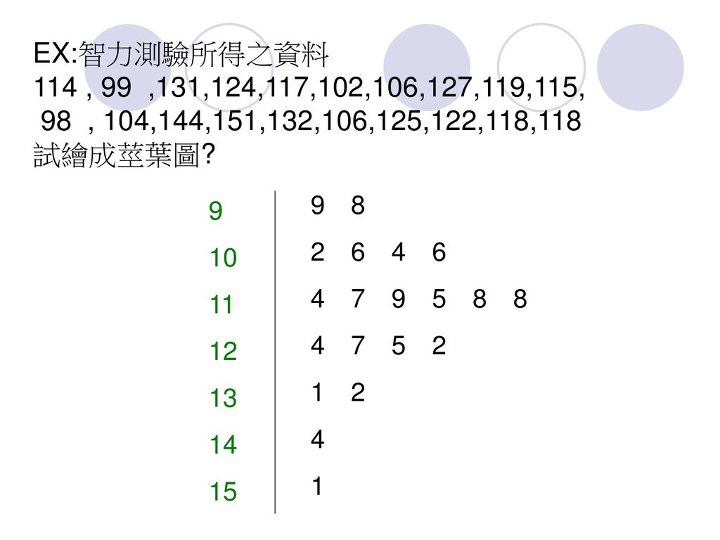
30 莖葉圖 (stem- and –leaf display)
探究性資料分析中可快速彙總資料且易繪製之圖形 優點:1.較直方圖易繪製 2.與直方圖相比，提供了更詳細的資料 繪製時，葉的部份(右邊)只用一個數字

31 EX:智力測驗所得之資料 114 , 99 ,131,124,117,102,106,127,119,115, 98 , 104,144,151,132,106,125,122,118,118 試繪成莖葉圖? 9　8 2　6　4　6 4　7　9　5　8　8 4　7　5　2 1　2 4 1 9 10 11 12 13 14 15

32 交叉表格（Crosstabulations)
交叉表格可用於兩個變數以上的資料彙總 表為300家餐廳的品質評等與餐點價格的交叉表格 餐點價格 品質評等 總和 $10-19　　$20-29　　$30-39　　$40-49 好 非常好 卓越 42　　　　　40　　　　2　　　　 0 34　　　　　64　　　　46　　　　6 2　　　　　 14　　　　28　　　　22 84 150 66 總和 78　　　　　118　　　 76　　　　28　 300

33 將表格中的次數轉換成百分比更能了解變數間的關係
表為品質評等類別的百分比 餐點價格 品質評等 總和 $10-19　　$20-29　　$30-39　　$40-49 好 非常好 卓越 50.0　　　　47.6　　　2.4　　　 0.0 22.7　　 　　　30.6　　　 4.0 3.0　　　　 21.2　　　42.4　　　33.4 100

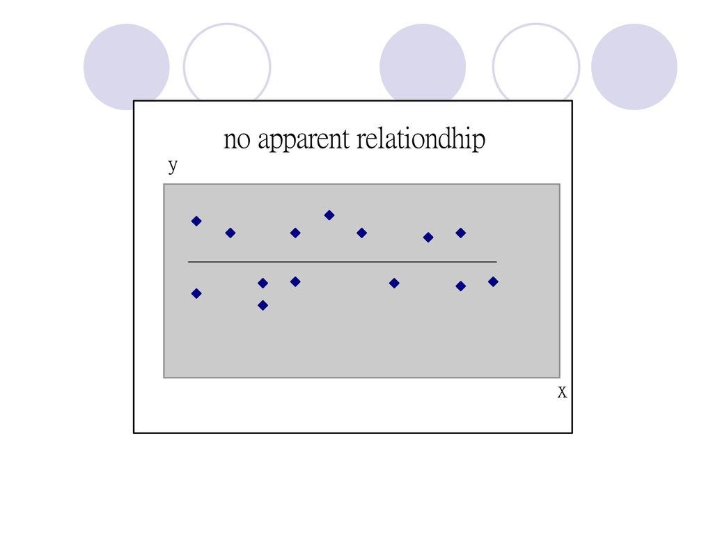
34 散佈圖(scatter diagram)與趨勢線(trendline)
散佈圖:表示兩定量變數間關係的圖 趨勢線:提供近似關係的直線 有正相關、負相關、沒有相關三種情形

35

36 Ex:以音響設備店的銷售量與廣告關係為例(教材P.49)
銷售量與廣告關係呈現正相關

37 數值 位置數量 離散數量 變異係數 全距 四分位數距 變異數 標準差 平均數 中位數 眾數 百分位數 四分位數

38 位置數量 Mean(平均數) Perhaps the most important measure of location is the mean. A measure of central location for the data. If the data are from a sample: x If the data are from a population: μ The mean is influenced by extremely small and large data values. Σx Σx i μ i 樣本平均數: x= 母體平均數: = n N (N表母體所包含的所有元素個數)

39 Ex:以下為五個大學班級的學生人數構成的樣本: 46 54 42 46 32
+ + + X + X X X X i 1 2 3 4 5 x= = = = 44 n 5 5 樣本平均數為44人

40 2.Median(中位數) The value in the middle when the data are arranged in ascending order (smallest value to largest value.) An odd number(奇數) of observations, the median is the middle value. An even number(偶數) of observations, the median is the average of the two middle values.

41 先將資料值由小到大排序 32,42,46,46,54 因為資料個數為奇數，故中位數=46
Ex1:求五個班級人數的中位數: 先將資料值由小到大排序 32,42,46,46,54 因為資料個數為奇數，故中位數=46

42 Ex2:商學院學生畢業起薪之中位數: middle two values = 2885 Median= 2

43 3.Mode(眾數) 資料集中出現次數最多的資料值 若資料中出現次數最多的值有兩個或兩個以上時，眾數就不只一個
出現兩個以上的眾數時，幾乎不被採用

44 在此處，眾數可用來表示最常被購買的飲料 EX:飲料購買狀況調查: Soft Drink Frequency Coke Classic 19
Diet Coke Dr. Pepper Pepsi-Cola Sprite total 在此處，眾數可用來表示最常被購買的飲料

45 4.Percentiles(百分位數) 瞭解資料在最小值與最大值間的分布情況 「百分之p 」表示至少有百分之p的觀察值會小於它

46 計算百分位數 1.Arrange the data in ascending order (smallest value to largest value). 2.Computer an index i i = x (p: percentile of interest, n :number of observations) 3.(a)If i is not an integer, round up.若非整數時,直接無條件進位取下一個數值 (b)If i is an integer, the pth is the average of the values in positions i and i+1.若為整數時,取其及下一個的平均數 p n 100

47 Ex: Determine the 85th percentile for the starting salary data.
Step 1 Step 2 i =( ) x 12=10.2 Step 3 Because i is not an integer, round up. The position of the 85th percentile is the next integer greater than 10.2 ,the 11th position,3130. 85 100

48 Another illustration of this procedure:
let us consider the calculation of the 50th percentile for the starting salary data . i=( )x12=6 因為i為整數,故取其及下一個數值的平均數,及取第6和第7個數字:( )/2=2905 85 100

49 5.Quartiles(四分位數) 將資料分為四個部份，每部份包含25%的觀察值
Q =first quartile ,or 25th percentile. Q =second quartile ,or 50th percentile. Q =third quartile ,or 75th percentile. 1 2 3

50 Ex:以下為起薪資料 Q =( )=2865 Q =( )=2905 1 2 Q =( )=3000 3

51 離散數量 1.Range(全距) 最簡單的離散量數—全距 計算方式:最大值-最小值 由於易受極端值影響，故不常使用
ex:我們用前頁的起薪資料來看，全距為 =615

52 2.Interquartile Range( IQR 四分位數距)
克服極端值的影響 計算簡單:IQR=Q -Q IQR為中間50%資料的全距 承前例，起薪的IQR= =135(中間50%的薪水差距約在135元左右) 3 1

53 3.Variance(變異數) 測偏離平均數的程度 母體變異數: 樣本變異數: σ= Σ(x -μ) N Σ(x -x ) S= n-1 2

54 Ex:班級人數資料之離差與離差平方的計算 (課本p.89)
平均班級人數 離差 離差的平方 2 (X ) (X) (X ) X (X ) X i i i 44 2 10 -2 -12 4 100 144 46 54 42 32 256 2 Σ(x -x ) 256 2 i S= = =64 n-1 4

55 4.Standard Deviation(標準差)
定義:變異數的正平方根 樣本標準差:s=√ 母體標準差:σ=√ 上頁提及班級人數樣本變異數 ，故樣本標準差為s=√ 2 s 2 σ 2 S=64 = 8 64

56 標準差與變異數的不同點 變異數經過平方，資料的單位不同無法比較 標準差單位與原始資料一致，可與同單位資料比較

57 5.Coefficient of Variation(變異係數)
為標準差相對於平均數的比例 變異係數:( )% 以班級人數為例，s=8，mean=44，則其變異係數為(8/44)x100%=18.2% 意即樣本標準差佔樣本平均數的18.2% Standard deviation X100 Mean

58 偏度(skewness) 次數分配不對稱程度 公式: Σ（ ） n X - X 3 i s (n-1)(n-2)

59 適度左偏 適度右偏 眾數>中位數>平均數 (右邊較多，故眾數最大) 眾數<中位數<平均數
(moderately skewed left) 適度右偏 (moderately skewed right) 眾數>中位數>平均數 (右邊較多，故眾數最大) 眾數<中位數<平均數

60 對稱(symmetric) 高度右偏 (highly skewed right) 中位數=平均數

61 z分數(z-scores) 為 與平均數之間有幾個標準差的差距 公式: z = 如:z =1.2表示x 比平均數多了約1.2個標準差 s
為 與平均數之間有幾個標準差的差距 公式: 如:z =1.2表示x 比平均數多了約1.2個標準差 X i X - X i z = i s 1 1 z = 第i項觀察值的z分數 樣本平均數 樣本標準差 i X = S =

62 Ex:公司部門員工數資料的z分數 公司部門員工數 離差 z分數 s (X - X) X - 2 10 -2 -12 2/8=0.25
i i i s 2 10 -2 -12 2/8=0.25 10/8=1.25 -2/8=-0.25 -12/8=-1.5 46 54 42 32 X=44 第五個觀察值的z分數為-1.5，表示其比平均數小1.5個標準差

63 柴比雪夫定理(Chebyshev’s Theorem)
2 任何資料集合內至少有(1-1/z )百分比的觀察值與平均數的差異在z個標準差之內 z必大於1 z=2,3,4時,運用柴比雪夫定理可知 至少有75%的觀察值與平均數的差距在2個標準差之內 至少有89%的觀察值與平均數的差距在3個標準差之內 至少有94%的觀察值與平均數的差距在4個標準差之內

64 Ex:某公司員工100人，年終評鑑分數平均為70分，標準差為5，試問:
1.有多少員工分數介於60~80之間? 2.有多少員工的分數介於58~82之間? Ans: 1.60和80分別小於和大於平均數2個標準差，根據柴比雪夫定理，至少有75%的觀察值與平均數的差距在2個標準差之內，因此，至少有75人的分數介於60~80間

65 2.(58-70)/5=-2.4 比平均數小2.4個標準差 (82-70)/5= 2.4 利用柴比雪夫定理z=2.4，可得
2.(58-70)/5=-2.4　　比平均數小2.4個標準差 (82-70)/5= 2.4 利用柴比雪夫定理z=2.4，可得 1-1/z = =0.826 至少有82.6%的員工平均分數介於58與82分 1 2 2 (2.4)

66 Empirical Rule(經驗法則) 許多實際應用的資料為鐘形分配
當資料趨近鐘形分配可利用經驗法則決定有多少百分比的觀察值與平均數的差距在某特定標準差之內 Bell-shaped distribution

67 Empirical Rule Approximately 68% of the data values will be within one standard deviation of the mean. Approximately 95% of the data values will be within two standard deviations of the mean. Almost all of the data values will be within three standard deviations of the mean.

68 Ex:生產出的巧克力重量通常為鐘形分配，若巧克力重量的平均數為每片160克，標準差是2.5克，由經驗法則可知:
1.約有68%的巧克力重量介於157.5與162.5克之間(與平均數的差距在一個標準差內) 2.約有95%的巧克力重量介於155與165克之間 3.幾乎所有的巧克力重量介於152.5與167.5克之間

69 Detecting Outliers(檢測極端值)
由經驗法則可知，資料若成鐘形分配，幾乎所有資料與平均數差距在三個標準差之內 以z分數檢測極端值: -3<z分數<3，若z分數超過此範圍就是極端值

70 Exploratory Data Analysis
利用簡單的算數與易繪之圖形來匯總資料，以下探討兩種方式: 1.Five–Number Summery(五數彙總) 2.Box Plot(箱形圖)

71 Five–Number Summery(五數彙總)
Smallest value First quartile (Q ) Median Third quartile (Q ) Largest value 將資料由左至右以遞增方式排列，馬上可得最小值、四分位數及最大值 1 3

72 Box Plot 根據五數彙總而繪製的圖形 關鍵:中位數與四分位數，也會用到 IQR(Q -Q ) 步驟:
1.以第一、三四分位數為前後邊(中間含50%資料) 2.箱形中的垂直線為中位數 3.箱子左右各推1.5個IQR為上下限(超過為極端值) 4.在上下限裡的max &min畫虛線表示 5.以*表示極端值 3 1

73 中位數 下界限 上界限 Q Q □ 3 1 * 1.5 (IQR) 1.5 (IQR) 極端值 IQR

74 Covariance(共變異數) Σ S = n-1 Σ μ σ = N 由於無法看出共變異數要多大才代表相關性很強，故少用之
(X - X) (y - y) i i 樣本共變異數: S = xy n-1 Σ (X -μ (y - μ ) ) i x i y 母體共變異數: σ = xy N 由於無法看出共變異數要多大才代表相關性很強，故少用之

75 正相關 負相關 S S Negative: (x and y are negatively linearly related)
Positive: (x and y are positively linearly related) xy xy

76 無相關 S Approximately 0: (x and y are not linearly related) xy

77 Correlation Coefficient(相關係數)
Pearson product moment correlation: sample data S xy r = ≦ 1 -1≦ s s xy x y r =sample correlation coefficient =sample covariance =sample standard deviation of x =sample standard deviation of y xy S xy s x s y

78 求相關係數? y X i i 先求平均數: 5　 10　　　30 15　　　50 X =( )/3=10 y =( )/3=45 S = 100 5 20 xy s x s y S xy The value of the sample correlation coefficient is 1 r =1 xy s s x y

79 若所有資料均落在一條正斜率的直線上，相關係數為+1，是完全正相關 若資料顯示x與y之間有正相關性但不是完全正相關，r 值會小於1

80 Weighted Mean(加權平均) x x w 當某些情況為了反映個別觀察值的重要性，計算平均數時要對每個觀察值加上權重 ΣW X i
加權平均數公式： = ΣW i x = value of observation i i w = weight for observation i i

81 Ex:以加權平均計算過去三個月購買原料之平均價格
Purchase　　　Cost per Pound　　　Number of Pounds　　　　　　 1　　　　　　3.0　　　　　　　　1100 2　　　　　　3.4　　　　　　　　500 3　　　　　　2.9　　　　　　　　2750 1100(3.0)+500(3.4)+2750(2.9) x = =2.983

82 Grouped Data(群組資料) 以下將示範如何從群組資料得出一些資訊 求群組資料的樣本平均數和樣本變異數? Frequency 4 8
稽核時間 (days) 10-14 15-19 20-24 25-29 30-34 Frequency 4 8 5 2 1 求群組資料的樣本平均數和樣本變異數? Total:

83 Σf M 380 樣本平均數:x= n 20 20 380 = = 19 天 i i i i 稽核時間(天) 10-14 15-19
20-24 25-29 30-34 組中點(M ) 12 17 22 27 32 次數(f ) 4 8 5 2 1 f M 4 8 5 2 1 i i i i 20 380 Σf M 380 i i 樣本平均數:x= = = 天 n 20

84 = =30 Σf (M -x ) n-1 570 19 20 570 樣本變異數: S = i i i i i i i 2 i i 2
196 32 45 128 169 次數 (f ) 4 8 5 2 1 離差 (M -x) -7 -2 3 8 13 離差的平方 (M -x) 49 4 9 64 169 i i 稽核時間 (天) 10-14 15-19 20-24 25-29 30-34 組中點 (M ) 12 17 22 27 32 i 2 i i i i 20 570 2 Σf (M -x ) 570 2 i i = 樣本變異數: S = =30 n-1 19

85 群組資料的母體變異數及母體平均數 2 Σf (M -μ) i i 2 母體變異數: σ = N Σf M μ 母體平均數: = i i N