Download presentation
Presentation is loading. Please wait.

1
operational research and optimize
经济模型与应用软件 运筹与优化 operational research and optimize 江西财经大学数学与管理工程系 华长生 电话: 课程网站: 论坛:

2
运筹与优化基本内容 1.线性规划的基本概念 2.线性规划与电子表格 3.线性规划的敏感性分析 4.运输与指派问题 5.网络最优化问题
6.整数优化与0—1规划 7.非线性规划 8.目标规划

3
Linear Programming: Basic Concepts
运筹与优化 1.线性规划的基本概念 Linear Programming: Basic Concepts

4
1.线性规划的基本概念 Session Topics An Class Working Example 一个课堂操作举例
Basic Concepts of Linear Programming 线性规划的基本概念 The Graphical Method for Solving LP 线性规划的图解法 Using Excel Solver to Solving 用微软Excel Solver 求解 Key Categories of LP Problems 线性规划问题的主要类型 Three Classic Applications of LP 三个经典的线性规划应用

5
The Lego Production Problem
1.线性规划的基本概念 1.1 一个简单例子 自己动手 The Lego Production Problem 拼装玩具生产 每个小组都有一组拼装玩具(8个小块和6 大块) ,这些是你们的原材料(raw materials),你们要用这些原材料去生产桌和椅( tables and chairs)这两种产品(products),具体拼装图如下一个幻灯片。 想想看! 你怎么去分析呢?
 ,这些是你们的原材料(raw materials),你们要用这些原材料去生产桌和椅( tables and chairs)这两种产品(products),具体拼装图如下一个幻灯片。 想想看! 你怎么去分析呢?")
6
1.线性规划的基本概念 原材料 产品 6 大块 8 小块 自己动手 桌 椅
桌 椅 利润(Profit) = $20/Table 利润 = $15/Chair
 = $20/Table 利润 = $15/Chair.")
7
1.线性规划的基本概念 自己动手 为了最小化成本或最大化利润的目的需要对一些稀缺资源进行配置 你的答案是什么?

8
Components of the Model
1.线性规划的基本概念 1.2 线性规划模型的构成 Components of the Model 模型的组成部分 Decision variables 决策变量 Objective function 目标函数 Constraints 约束

9
Assumptions of Linear Programming
1.线性规划的基本概念 Assumptions of Linear Programming 线性规划的假设 Linearity 线性 Divisibility 可分性 Certainty 确定性 Nonnegativity 非负性

10
Why Use Linear Programming?
1.线性规划的基本概念 Why Use Linear Programming? 为什么要使用线性规划 线性规划很容易而有效率地被求解 如果存在最优解,则肯定能够找到 功能强大的敏感性分析(sensitivity analysis) 许多实际问题本质上是线性的
 许多实际问题本质上是线性的.")
11
Mathematical Statement of LP Problem
1.线性规划的基本概念 Mathematical Statement of LP Problem 线性规划的数学描述 线性规划要确定决策变量 x1, x2, … , xn 使得 已知参数 c1, … , cn ; a11, … , amn ; b1, … , bm.

12
Steps in Formulating LP Problem
1.线性规划的基本概念 Steps in Formulating LP Problem 线性规划问题建模步骤 需要做哪些决策?决策变量是什么 问题的目标是什么?写出目标函数 资源和需求之间的情况如何? 确定约束条件

13
The Graphical Method for Solving LP
1.线性规划的基本概念 1.3 线性规划模型的理论解法 T=3-0.75c The Graphical Method for Solving LP 线性规划的图解法

14
The Simple Method for Solving LP
1.线性规划的基本概念 The Simple Method for Solving LP 线性规划的单纯形法

15
The Art of Modeling with Spreadsheets
运筹与优化 2.线性规划与电子表格 The Art of Modeling with Spreadsheets

16
Using Excel Solver to Solving
2.线性规划与电子表格 2.1 Excel Solver的安装 Using Excel Solver to Solving 用微软Excel Solver 求解

17
Solving Lego Problem 求解玩具拼装问题
2.线性规划与电子表格 2.2 Excel Solver的使用 Solving Lego Problem 求解玩具拼装问题 用易理解方式输入数据和构筑数据之间的联系 定义目标单元格(目标函数) 确定可变单元(决策变量) 添加约束变量(Adding Constraints)
 确定可变单元(决策变量) 添加约束变量(Adding Constraints)")
18
2.2 Excel Solver的使用

19
2.线性规划与电子表格 The Solution 求解结果

20
Key Categories of LP Problems
2.线性规划与电子表格 2.3 建模与应用 Key Categories of LP Problems 线性规划问题主要类型 资源分配问题(resource-allocation) 成本收益平衡问题 (cost-benefit-trade-off) 网络配送问题(distribution-network) 混合问题(mixed Problem)
 成本收益平衡问题 (cost-benefit-trade-off) 网络配送问题(distribution-network) 混合问题(mixed Problem)")
21
Resource-allocation Problem资源分配问题
2.线性规划与电子表格 问题类型1 Resource-allocation Problem资源分配问题 资源分配(resource-allocation)问题是将有限的资源 分配到各种活动中去的线性规划问题。这一类问题的 共性是在线性规划模型中每一个函数限制均为资源限 制(resource constraint) , 并且每一种有限资源都可以表 现为如下的形式: 使用的资源数量 可用的资源数量
问题是将有限的资源. 分配到各种活动中去的线性规划问题。这一类问题的. 共性是在线性规划模型中每一个函数限制均为资源限. 制(resource constraint) , 并且每一种有限资源都可以表. 现为如下的形式: 使用的资源数量 可用的资源数量.")
22
2.线性规划与电子表格 Datum Gathering 收集数据 所有活动可获得使用的每种资源的有限数量
每一种活动所需要的各种资源的数量, 每一种资源 与活动的组合,单位活动消耗资源量必须首先估计 每一种活动对总的绩效测度的单位贡献

23
Super Grain Corp. 超级谷物公司
2.线性规划与电子表格 实际举例1 Super Grain Corp. 超级谷物公司 超级谷物公司为了大规模进入已有许多供应商的早 点谷物类食品市场,雇佣了一家广告公司设计全国 性的促销活动,广告设计费用不超过100万美元, 广告传播费用不超过400万美元。 广告媒介: 媒介1:星期六上午儿童节目的电视广告 媒介2:食品与家庭导向杂志上的广告 媒介3:主要报纸星期天增刊上的广告

24
Super Grain Corp. 超级谷物公司
2.线性规划与电子表格 Super Grain Corp. 超级谷物公司 超级谷物公司广告组合问题的成本和广告受众数据 成本类型 成本(美元) 每次电视广告 每份杂志广告 每份增刊广告 广告受众期望量 ,300, , ,000 1. 广告传播预算 , , ,000 2. 规划设计预算 , , ,000 儿童节目的电视广告资源紧张,只有5个广 告时段可以使用,其他广告资源数量不限 如何组合, 受众最大?
 每次电视广告. 每份杂志广告. 每份增刊广告. 广告受众期望量 1,300, , , 广告传播预算 300, , , 规划设计预算 90,000 30,000 40,000. 儿童节目的电视广告资源紧张,只有5个广. 告时段可以使用,其他广告资源数量不限. 如何组合, 受众最大")
25
Super Grain Corp. 超级谷物公司
2.线性规划与电子表格 Super Grain Corp. 超级谷物公司 资源限制: 资源1:广告传播预算400万美元 资源2:广告规划设计预算100万美元 资源3:可获得的儿童节目的电视广告只有5个时段 单位: 万美元 万人

26
2.线性规划与电子表格 Super Grain Corp. 超级谷物公司

27
Think-Big Development Co.
2.线性规划与电子表格 实际举例2 梦大发展公司 Think-Big Development Co. 梦大发展公司是商务房地产项目的主要投资商,现 该公司有机会在三个投资项目中投资: 项目1:建造高层办公楼 项目2:建造宾馆 项目3:建造购物中心 公司的资金来源:现有2500万美元,预计一年后可获 得2000万美元,两年后可再获得2000万美元,三年后 又可获得1500万美元

28
Think-Big Development Co.
2.线性规划与电子表格 Think-Big Development Co. 梦大发展公司 梦大发展公司部分投资项目的财务数据 年份 所需投资资金成本(百万美元) 办公楼项目 宾馆项目 购物中心项目 净现值(收益) 梦大公司不必投资整个项目,可以按比例进行投 资,梦大公司的决策者如何决策,使净现值最大?
 办公楼项目. 宾馆项目. 购物中心项目. 净现值(收益) 梦大公司不必投资整个项目,可以按比例进行投. 资,梦大公司的决策者如何决策,使净现值最大?")
29
Think-Big Development Co.
2.线性规划与电子表格 Think-Big Development Co. 梦大发展公司 梦大发展公司的投资组合问题资源数据表 0(现在) 1(1年后) 2(2年后) 3(3年后) 资源 每种投资累计资金需求量(百万美元) 办公楼项目 宾馆项目 购物中心项目 可获得资金数
 (1年后) (2年后) (3年后) 资源. 每种投资累计资金需求量(百万美元) 办公楼项目. 宾馆项目. 购物中心项目. 可获得资金数.")
30
Think-Big Development Co.
2.线性规划与电子表格 Think-Big Development Co. 梦大发展公司

31
Cost-benefit-trade-off Problem
2.线性规划与电子表格 问题类型2 Cost-benefit-trade-off Problem 成本收益平衡问题 成本收益平衡问题( Cost-benefit-trade-off Problem ) 是一类线性规划问题,这类问题中,通过选择各种 活动水平的组合,从而以最小的成本来实现最低可 接受的各种收益的水平。这类问题的共性是,所有 的函数约束均为收益约束,并具有如下的形式: 完成的水平 最低可接受的水平
 是一类线性规划问题,这类问题中,通过选择各种. 活动水平的组合,从而以最小的成本来实现最低可. 接受的各种收益的水平。这类问题的共性是,所有. 的函数约束均为收益约束,并具有如下的形式: 完成的水平 最低可接受的水平.")
32
Union Airways Corp. 联合航空公司
2.线性规划与电子表格 Union Airways Corp. 联合航空公司 实际举例3 联合航空公司计划增加其中心机场的往来航班, 需要 雇佣更多的客户代理商。按照公司与代理商的协议, 要求 每个代理商工作8小时为一班,共有5个不同时段的轮班 如下: 轮班1: 6:00 AM to 2:00 PM 轮班2: 8:00 AM to 4:00 PM 轮班3: Noon to 8:00 PM 轮班4: 4:00 PM to midnight 轮班5: 10:00 PM to 6:00 AM 问题: 每个时段应该雇佣多少代理商?

33
Union Airways Corp. 联合航空公司
2.线性规划与电子表格 Union Airways Corp. 联合航空公司 轮班的时段 时段 1 2 3 4 5 代理商的最小数量 6 AM to 8 AM √ 48 8 AM to 10 AM 79 10 AM to noon 65 Noon to 2 PM 87 2 PM to 4 PM 64 4 PM to 6 PM 73 6 PM to 8 PM 82 8 PM to 10 PM 43 10 PM to midnight 52 Midnight to 6 AM 15 代理商的轮班成本 $170 $160 $175 $180 $195

34
Union Airways Corp. 联合航空公司
2.线性规划与电子表格 Union Airways Corp. 联合航空公司 轮班的时段 时段 1 2 3 4 5 代理商的最小数量 6 AM to 8 AM √ 48 8 AM to 10 AM 79 10 AM to noon 65 Noon to 2 PM 87 2 PM to 4 PM 64 4 PM to 6 PM 73 6 PM to 8 PM 82 8 PM to 10 PM 43 10 PM to midnight 52 Midnight to 6 AM 15 代理商的轮班成本 $170 $160 $175 $180 $195 S1 ≥ 48 S1 + S2 ≥ 79 S1 + S2 ≥ 65 S1 + S2 + S3 ≥ 87 S2 + S3 ≥ 64 S3 + S4 ≥ 73 S3 + S4 ≥ 82 S4 ≥ 43 S4 + S5 ≥ 52 S5 ≥ 15

35
Union Airways Corp. 联合航空公司
2.线性规划与电子表格 Union Airways Corp. 联合航空公司 设 Si 为轮班 i 的数量 ( i = 1 to 5), Minimize Cost = $170S1 + $160S2 + $175S3 + $180S4 + $195S5 subject to Total agents 6AM–8AM: S1 ≥ 48 Total agents 8AM–10AM: S1 + S2 ≥ 79 Total agents 10AM–12PM: S1 + S2 ≥ 65 Total agents 12PM–2PM: S1 + S2 + S3 ≥ 87 Total agents 2PM–4PM: S2 + S3 ≥ 64 Total agents 4PM–6PM: S3 + S4 ≥ 73 Total agents 6PM–8PM: S3 + S4 ≥ 82 Total agents 8PM–10PM: S4 ≥ 43 Total agents 10PM–12AM: S4 + S5 ≥ 52 Total agents 12AM–6AM: S5 ≥ 15 and Si ≥ 0 (for i = 1 to 5)
, Minimize Cost = $170S1 + $160S2 + $175S3 + $180S4 + $195S5 subject to Total agents 6AM–8AM: S1 ≥ 48 Total agents 8AM–10AM: S1 + S2 ≥ 79 Total agents 10AM–12PM: S1 + S2 ≥ 65 Total agents 12PM–2PM: S1 + S2 + S3 ≥ 87 Total agents 2PM–4PM: S2 + S3 ≥ 64 Total agents 4PM–6PM: S3 + S4 ≥ 73 Total agents 6PM–8PM: S3 + S4 ≥ 82 Total agents 8PM–10PM: S4 ≥ 43 Total agents 10PM–12AM: S4 + S5 ≥ 52 Total agents 12AM–6AM: S5 ≥ 15 and Si ≥ 0 (for i = 1 to 5)")
36
2.线性规划与电子表格 Union Airways Corp. 联合航空公司

37
Distribution-network Problem
2.线性规划与电子表格 问题类型3 Distribution-network Problem 网络配送问题 网络配送问题(distribution network)能以最小的成 本完成货物的配送,所以称之为网络配送问题并具有 如下的确定性约束形式: 提供的数量=需要的数量 提供的数量>=需要的数量
能以最小的成. 本完成货物的配送,所以称之为网络配送问题并具有. 如下的确定性约束形式: 提供的数量=需要的数量. 提供的数量>=需要的数量.")
38
Distribution Unlimited Co.
2.线性规划与电子表格 实际举例4 Distribution Unlimited Co. 无限配送公司 大M公司在两个工厂生产多种重型机械设备,其中一种就 是大型六角车床,公司有三个客户需要这种六角车床。公 司委托无限配送公司运送这些车床。 问题:每个工厂要运送多少车床到每个客户?

39
Distribution Unlimited Co.
2.线性规划与电子表格 Distribution Unlimited Co. 无限配送公司 每台车床的运输成本 To 客户1 客户2 客户3 From 产量 工厂1 $700 $900 $800 12 lathes 工厂2 800 900 700 15 lathes 需求量 10 lathes 8 lathes 9 lathes 提供的数量=需要的数量

40
Distribution Unlimited Co.
2.线性规划与电子表格 Distribution Unlimited Co. 无限配送公司 提供的数量=需要的数量

41
Distribution Unlimited Co.
2.线性规划与电子表格 Distribution Unlimited Co. 无限配送公司 Let Sij = Number of lathes to ship from i to j (i = F1, F2; j = C1, C2, C3). Minimize Cost = $700SF1-C1 + $900SF1-C2 + $800SF1-C $800SF2-C1 + $900SF2-C2 + $700SF2-C3 subject to Factory 1: SF1-C1 + SF1-C2 + SF1-C3 = 12 Factory 2: SF2-C1 + SF2-C2 + SF2-C3 = 15 Customer 1: SF1-C1 + SF2-C1 = 10 Customer 2: SF1-C2 + SF2-C2 = 8 Customer 3: SF1-C3 + SF2-C3 = 9 and Sij ≥ 0 (i = F1, F2; j = C1, C2, C3).
. Minimize Cost = $700SF1-C1 + $900SF1-C2 + $800SF1-C3 + $800SF2-C1 + $900SF2-C2 + $700SF2-C3 subject to Factory 1: SF1-C1 + SF1-C2 + SF1-C3 = 12 Factory 2: SF2-C1 + SF2-C2 + SF2-C3 = 15 Customer 1: SF1-C1 + SF2-C1 = 10 Customer 2: SF1-C2 + SF2-C2 = 8 Customer 3: SF1-C3 + SF2-C3 = 9 and Sij ≥ 0 (i = F1, F2; j = C1, C2, C3).")
42
Distribution Unlimited Co.
2.线性规划与电子表格 Distribution Unlimited Co. 无限配送公司

43
2.线性规划与电子表格 混合问题 Mixed Problem
问题类型4 混合问题 Mixed Problem 资源分配问题,成本收益平衡问题以及网络配送问题,都以一类约束条件为特色的。实际上,纯资源分配问题的共性是它所有的函数约束均为资源约束,而成本收益平衡问题的共性是它所有的函数约束均为收益约束,网络配送问题中,主要的函数约束为一特定类型的确定需求的约束。 混合问题 是第四类线性规划问题,这一类型包括 了三类约束函数

44
2.线性规划与电子表格 塞维特公司 Save-It Company 塞维特公司经营一家回收中心,该中心专门回收4种
实际举例5 塞维特公司经营一家回收中心,该中心专门回收4种 固体废弃物,并将废弃物进行处理混合成可以销售的 小产品,根据混合时废弃物的不同比例,可生产三种 不同等级的产品:A, B,和 C。 问题:每种废弃物各使用多少,三种产品各生产多少 使利润最大?

45
2.线性规划与电子表格 塞维特公司 Save-It Company 5.50 2.00 材料1: 不超过总量的70% C 7.00 2.50
材料1: 不超过总量的50% 材料2: 不少于总量的10% 材料4: 总量的10% B $8.50 $3.00 材料1: 不超过总量的30% 材料2: 不少于总量的40% 材料3: 不超过总量的50% 材料4: 总量的20% A 每磅售价 每磅混合 成本 规格说明 等级

46
2.线性规划与电子表格 塞维特公司 Save-It Company 材料 每周可获得量 (磅) 每磅处理成本( 美元) 附加约束 1
3,000 $3.00 1. 对每种材料,每周必须回收并处理一半. 2. 每周$30,000用于处理这些材料. 2 2,000 6.00 3 4,000 4.00 4 1,000 5.00

47
2.线性规划与电子表格 Save-It Company 塞维特公司
Let xij = Pounds of material j allocated to product i per week (i = A, B, C; j = 1, 2, 3, 4). Maximize Profit = 5.5(xA1 + xA2 + xA3 + xA4) + 4.5(xB1 + xB2 + xB3 + xB4) + 3.5(xC1 + xC2 + xC3 + xC4) subject to Mixture Specifications: xA1 ≤ 0.3 (xA1 + xA2 + xA3 + xA4) xA2 ≥ 0.4 (xA1 + xA2 + xA3 + xA4) xA3 ≤ 0.5 (xA1 + xA2 + xA3 + xA4) xA4 = 0.2 (xA1 + xA2 + xA3 + xA4) xB1 ≤ 0.5 (xB1 + xB2 + xB3 + xB4) xB2 ≥ 0.1 (xB1 + xB2 + xB3 + xB4) xB4 = 0.1 (xB1 + xB2 + xB3 + xB4) xC1 ≤ 0.7 (xC1 + xC2 + xC3 + xC4) Availability of Materials: xA1 + xB1 + xC1 ≤ 3,000 xA2 + xB2 + xC2 ≤ 2,000 xA3 + xB3 + xC3 ≤ 4,000 xA4 + xB4 + xC4 ≤ 1,000 Restrictions on amount treated: xA1 + xB1 + xC1 ≥ 1,500 xA2 + xB2 + xC2 ≥ 1,000 xA3 + xB3 + xC3 ≥ 2,000 xA4 + xB4 + xC4 ≥ 500 Restriction on treatment cost: 3(xA1 + xB1 + xC1) + 6(xA2 + xB2 + xC2) (xA3 + xB3 + xC3) + 5(xA4 + xB4 + xC4) = 30, and xij ≥ 0 (i = A, B, C; j = 1, 2, 3, 4). Save-It Company 塞维特公司
. Maximize Profit = 5.5(xA1 + xA2 + xA3 + xA4) + 4.5(xB1 + xB2 + xB3 + xB4) + 3.5(xC1 + xC2 + xC3 + xC4) subject to Mixture Specifications: xA1 ≤ 0.3 (xA1 + xA2 + xA3 + xA4) xA2 ≥ 0.4 (xA1 + xA2 + xA3 + xA4) xA3 ≤ 0.5 (xA1 + xA2 + xA3 + xA4) xA4 = 0.2 (xA1 + xA2 + xA3 + xA4) xB1 ≤ 0.5 (xB1 + xB2 + xB3 + xB4) xB2 ≥ 0.1 (xB1 + xB2 + xB3 + xB4) xB4 = 0.1 (xB1 + xB2 + xB3 + xB4) xC1 ≤ 0.7 (xC1 + xC2 + xC3 + xC4) Availability of Materials: xA1 + xB1 + xC1 ≤ 3,000 xA2 + xB2 + xC2 ≤ 2,000 xA3 + xB3 + xC3 ≤ 4,000 xA4 + xB4 + xC4 ≤ 1,000 Restrictions on amount treated: xA1 + xB1 + xC1 ≥ 1,500 xA2 + xB2 + xC2 ≥ 1,000 xA3 + xB3 + xC3 ≥ 2,000 xA4 + xB4 + xC4 ≥ 500 Restriction on treatment cost: 3(xA1 + xB1 + xC1) + 6(xA2 + xB2 + xC2) + 4(xA3 + xB3 + xC3) + 5(xA4 + xB4 + xC4) = 30,000 and xij ≥ 0 (i = A, B, C; j = 1, 2, 3, 4). Save-It Company. 塞维特公司.")
48
2.线性规划与电子表格 塞维特公司 Save-It Company 实际举例5

49
2.线性规划与电子表格 塞维特公司 Save-It Company

50
2.线性规划与电子表格 塞维特公司 Save-It Company 变量名称的定义

51
Summary of LP Types 线性规划问题总结
2.线性规划与电子表格 2.4 类型总结 Summary of LP Types 线性规划问题总结 类型 形式 解释 主要用于 资源约束 LHS RHS 对于特定的资源使用的数量 可获得的数量 资源分配问题混合问题 收益约束 LHS RHS 对于特定的收益达到的水平 最低可接受水平 成本收益平衡问题混合问题 需求确定约束 LHS=RHS 对于一些数量提供的数量= 需求的数量 网络配送问题混合问题

52
Classical Applications of LP
2.线性规划与电子表格 应用回顾 Classical Applications of LP 线性规划经典应用回顾 为潘德罗索工业公司选择产品组合 联合航空公司工作人员排程 Citgo石油集团供应、配送 与营销的规划

53
Ponderosa Industrial 潘德罗索工业公司
2.线性规划与电子表格 公司经验 Ponderosa Industrial 潘德罗索工业公司 潘德罗索应用成功的因素: 以自然语言为用户界面的财务计划系统,使用自然语言而不是数学符号来显示线性规划模型各个组成部分以及输出的结果,使得做决策的管理者能够很容易看懂整个过程。 最优化系统是互动的(interactive),管理者在从一个版本的模型中获得一组最优解之后,可以提出一系列的what-if问题,并能立即得到回应。
,管理者在从一个版本的模型中获得一组最优解之后,可以提出一系列的what-if问题,并能立即得到回应。")
54
Personnel Scheduling at UA.
2.线性规划与电子表格 公司经验 Personnel Scheduling at UA. 联合航空公司人员排程 联合航空公司 利用线性规划,来为其在主要的机场和订票点的上万个工作人员安排每周的工作时间表。目标是为了能够在满足客户的服务需要的同时,将一周内每天每半个小时的人员成本最小化。联合航空公司一些地点的规划模型却包括20,000个决策变量。 应用成功最主要的因素是因为得到了运营经理以及其它员工的大力支持。

55
Citgo Petroleum Corporation
2.线性规划与电子表格 公司经验 Citgo Petroleum Corporation Citgo石油集团 Citgo石油集团 运用管理科学的技术,特别是线性规划,建立供应、配送与营销的建模系统将公司主要产品的供应、配送与营销通过公司庞大的销售与配送网络得到很好的协调。在90年代中期创造了大量的财富。 公司每种主要产品的模型都含有大约1,500个决策量以及3,000个确定需求的约束 最重要的成功因素是高层管理者所给予的无限制的支持,并且设立运作协调副总裁,来负责评价与协调这一跨组织边界的模型所提供的建议

56
2.线性规划与电子表格 Session Summary 本讲小结
以符号表示的函数约束称为资源约束,这些限制要求使用的资源必须小于等于所能提供的资源的数量。资源分配问题的共性就是它们的函数约束全部为资源约束。 以符号表示的函数约束为收益约束,形式为收益取得的水平必须大于等于最低可接受水平。收益约束反映了管理层所规定的目标。如果所有约束均为收益约束,这一问题为成本收益平衡问题。

57
2.线性规划与电子表格 Session Summary 本讲小结
以=符号表示的函数约束称为确定需求的约束,它们表示了一定数量的确定的需求,提供的数量等于要求的数量。网络配送问题的共性就是它们的主要函数约束为一种特定形式的确定需求的约束。 不能归于这三类的任何线性规划的问题称为混合问题。 在实际的应用当中,管理科学小组经常建立和分析大型的线性规划模型以指导管理决策,这些工作需要管理层足够强大的管理上的投入与支持,才能达到管理层实际的要求。

58
Sensitivity Analysis and It’s Applications
运筹与优化 3. 敏感性分析及其应用 Sensitivity Analysis and It’s Applications

59
3.线性规划的敏感性分析 Session Topics What is Sensitivity Analysis 什么是敏感性分析
The Importance of What-If Analysis to Managers 敏感性分析对管理者的重要性 Wyndor Case Study 伟恩德公司案例研究 Range-of-Optimality What-If Analysis 最优域敏感性分析

60
3.线性规划的敏感性分析 Session Topics 1. 什么是敏感性分析 Simultaneous Change in OFC
同时改变目标函数系数 Shadow Price Analysis for RHS 右端项的影子价格分析 Range-of-Feasibility What-If Analysis 可行域的敏感性分析 Simultaneous Change in RHS 同时改变右端项

61
The Lego Production Problem
3.线性规划的敏感性分析 3.1 什么是敏感性分析 自己动手 The Lego Production Problem 拼装玩具生产 如果桌子的利润是$35,最优解会怎样变化呢? 如果又有一个额外的大块,会增加总利润吗? 如果桌子和椅子构成改变,最优解会变化吗? 如果有一些原材料,你愿意以多大的代价 购买呢? 想想看! 你怎么来分析这些问题?

62
What is Sensitivity Analysis
3.线性规划的敏感性分析 What is Sensitivity Analysis 什么是敏感性分析 数学模型只是实际问题的一个粗略的抽象 最优解一般只是针对某一特定的数学模型 管理者要对未来做各种假设,在这些假设下,测试可能产生的结果,通过对各种结果深入分析来指导决策 通常,在取得最初版本模型的最优解之后,进行分析才能取得对问题深入的认识 这种分析称为what-if分析 或敏感性分析(Sensitivity Analysis)
")
63
The Importance of What-If Analysis to Managers
3.线性规划的敏感性分析 The Importance of What-If Analysis to Managers 敏感性分析对管理者的重要性 模型参数是粗略的估计值 获取所需数据必须付出相当多的时间与心血 有些因素只有在研究完成后才能精确测量 what-if分析可以表明改变这些决策对结果的影响,从而有效指导管理者作出最终的决策

64
3.线性规划的敏感性分析 3.2 Wyndor公司案例研究 Wyndor玻璃制品公司开发了两种新产品: 8英尺的铝框玻璃门
4X6英尺的双把木框窗 公司有3个工厂: 工厂1生产铝框和五金配件 工厂2生产木框 工厂3加工玻璃和组装门和窗 问题: 公司是否应该生产这两种新产品? 如果生产,应该如何生产,每周应该生产多少?

65
Wyndor Case Study 伟恩德公司案例研究
3.线性规划的敏感性分析 Wyndor Case Study 伟恩德公司案例研究 基本数据

66
Wyndor Case Study 伟恩德公司案例研究
3.线性规划的敏感性分析 Wyndor Case Study 伟恩德公司案例研究 Let D = the number of doors to produce W = the number of windows to produce Maximize P = $300D + $500W subject to D ≤ W ≤ 12 3D + 2W ≤ 18 and D ≥ 0, W ≥ 0.

67
Wyndor Case Study 伟恩德公司案例研究
3.线性规划的敏感性分析 Wyndor Case Study 伟恩德公司案例研究 原问题最优解 利润 产品组合

68
Wyndor Case Study 伟恩德公司案例研究
3.线性规划的敏感性分析 Wyndor Case Study 伟恩德公司案例研究 门的单位利润从$300下降到$200,最优解没有改变, 但利润下降 利润 产品组合

69
Wyndor Case Study 伟恩德公司案例研究
3.线性规划的敏感性分析 Wyndor Case Study 伟恩德公司案例研究 门的单位利润从$300上升到$500,最优解没有改变, 但利润也上升 利润 产品组合

70
Wyndor Case Study 伟恩德公司案例研究
3.线性规划的敏感性分析 Wyndor Case Study 伟恩德公司案例研究 门的单位利润从$300上升到$1000,最优解也随着改 变,利润也上升 利润 产品组合

71
3.线性规划的敏感性分析 3.3 用Solver Table宏作敏感性分析 Solver Table宏的安装使用
1.Be sure that the Solver is installed. If it is, it should appear under the Tools menu. If it is not, use the Excel or Microsoft Office installation CD to install it 2.Quit Excel if it is currently running. 3.Save the Solver Table.xla file to the exact same location as the Solver.xla file (see file info in box below). a. On a PC, this will typically be at C:\program files\Microsoft Office\ Office\Library\Solver\Solver.xla. (If it is not, use the Find command to find the Solver.xla file). b. On a Macintosh this will typically be in the Microsoft Office: Office:Add-Ins folder. (If it is not, use Find File or Sherlock to locate the Solver.xla file.) 4.Launch Excel. 5.Under the Tools menu, choose the "Add-Ins" command. 6.Click the Solver Table checkbox to have Solver Table load with Excel every time it is loaded. (Uncheck the box to have Solver Table not load next time Excel is launched.)
. a. On a PC, this will typically be at C:\program files\Microsoft Office\ Office\Library\Solver\Solver.xla. (If it is not, use the Find command. to find the Solver.xla file). b. On a Macintosh this will typically be in the Microsoft Office: Office:Add-Ins folder. (If it is not, use Find File or Sherlock to locate. the Solver.xla file.) 4.Launch Excel. 5.Under the Tools menu, choose the Add-Ins command. 6.Click the Solver Table checkbox to have Solver Table load with. Excel every time it is loaded. (Uncheck the box to have Solver. Table not load next time Excel is launched.)")
72
Wyndor Case Study 伟恩德公司案例研究
3.线性规划的敏感性分析 Wyndor Case Study 伟恩德公司案例研究 (1) 只有一个目标函数系数变动时的影响 门的单位利润从$100变到$1000,产品组合的变化
 只有一个目标函数系数变动时的影响. 门的单位利润从$100变到$1000,产品组合的变化.")
73
Wyndor Case Study 伟恩德公司案例研究
3.线性规划的敏感性分析 Wyndor Case Study 伟恩德公司案例研究 门的单位利润从$700变到$790,产品组合的变化

74
Wyndor Case Study 伟恩德公司案例研究
3.线性规划的敏感性分析 Wyndor Case Study 伟恩德公司案例研究 最优解(产品组合)不变的前提下,门(或窗)的利润 值允许变化的范围
不变的前提下,门(或窗)的利润. 值允许变化的范围.")
75
3.线性规划的敏感性分析 (2) 目标函数系数同时变动的影响
如何在不重新求解模型的条件下,确定如果目标函数的几个系数同时变化,可能造成对最优解的影响 如果伟恩德公司两种新产品单位利润的估计值都是不精确的,将会对结果产生怎样的影响?

76
Wyndor Case Study 伟恩德公司案例研究
3.线性规划的敏感性分析 Wyndor Case Study 伟恩德公司案例研究 修正的Wyndor问题模型,其中门,窗的单位利润分别被改为PD=$450,PW=$400,但是最优解不变

77
Wyndor Case Study 伟恩德公司案例研究
3.线性规划的敏感性分析 Wyndor Case Study 伟恩德公司案例研究 修正的Wyndor问题模型,其中门,窗的单位利润分别被改为PD=$600,PW=$300,从而最优解改变

78
Wyndor Case Study 伟恩德公司案例研究
3.线性规划的敏感性分析 Wyndor Case Study 伟恩德公司案例研究 伟恩德例子中系统改变门,窗单位利润得到的数据表

79
The 100 percent rule 百分之百法则
3.线性规划的敏感性分析 (3) 百分百法则 The 100 percent rule 百分之百法则 目标函数系数同时变动的百分之百法则: 如果目标函数的系数同时变动,计算出每一系数变动量占该系数最优域允许变动量的百分比,而后,将各个系数的变动百分比相加,如果所得之和不超过百分之一百,最优解不会改变,如果超过百分之一百,则不能确定最优解是否改变。
 百分百法则. The 100 percent rule. 百分之百法则. 目标函数系数同时变动的百分之百法则: 如果目标函数的系数同时变动,计算出每一系数变动量占该系数最优域允许变动量的百分比,而后,将各个系数的变动百分比相加,如果所得之和不超过百分之一百,最优解不会改变,如果超过百分之一百,则不能确定最优解是否改变。")
80
Wyndor Case Study 伟恩德公司案例研究
3.线性规划的敏感性分析 Wyndor Case Study 伟恩德公司案例研究 W D 2 4 6 8 可行域 10 (4, 3) (2, 6) 窗户 的每 周产 量 门的每周产量 P =300D +500W
 (2, 6) 窗户. 的每. 周产. 量. 门的每周产量. P =300D +500W.")
81
Role of the 100 percent rule
3.线性规划的敏感性分析 Role of the 100 percent rule 百分之百法则的作用 可用于确定在保持最优解不变的条件下,目标函 数系数的变动范围 百分百法则通过将允许的增加或减少值在各个系 数之间分摊,从而可以直接显示出每个系数的允 许变动值 线性规划研究结束以后,如果将来条件变 化,致 使目标函数中一部分或所有系数都发生变动,百 分百法则可以直接表明最初最优解是否保持不变

82
Shadow Price Analysis for RHS
3.线性规划的敏感性分析 (4) 单个约束条件变化的影响 右端项的影子价格分析 Shadow Price Analysis for RHS 分析函数约束右端值变动的原因是不能得到模型的 参数的精确值,只能对其作大略的估计。因此要知 道万一这些估计不准确产生的后果 更主要的理由是因为这些常数往往不是由外界决定 的而是管理层的政策决策。在建模并求解后,管理 者想要知道如果改变这些决策是否会提高最终收益 影子价格分析就是为管理者提供这方面的信息
 单个约束条件变化的影响. 右端项的影子价格分析. Shadow Price Analysis for RHS. 分析函数约束右端值变动的原因是不能得到模型的. 参数的精确值,只能对其作大略的估计。因此要知. 道万一这些估计不准确产生的后果. 更主要的理由是因为这些常数往往不是由外界决定. 的而是管理层的政策决策。在建模并求解后,管理. 者想要知道如果改变这些决策是否会提高最终收益. 影子价格分析就是为管理者提供这方面的信息.")
83
3.线性规划的敏感性分析 Shadow Price 影子价格

84
Wyndor Case Study 伟恩德公司案例研究
3.线性规划的敏感性分析 Wyndor Case Study 伟恩德公司案例研究 工厂2每周提供的生产时间从12小时增加到13小时, 总利润每周增加$150 per week.

85
Wyndor Case Study 伟恩德公司案例研究
3.线性规划的敏感性分析 Wyndor Case Study 伟恩德公司案例研究 工厂2每周提供的生产时间从13小时增加到18小时, 总利润每周增加$750(每小时增加$150)
")
86
Wyndor Case Study 伟恩德公司案例研究
3.线性规划的敏感性分析 Wyndor Case Study 伟恩德公司案例研究 工厂2每周提供的生产时间从18小时增加到20小时, 总利润不再进一步增加

87
The Message to Management
3.线性规划的敏感性分析 The Message to Management 给管理层的信息 给管理层的信息:影子价格被定义为,线性规划的函数约束右端值每增加一个单位,所引起的目标函数值的增加。但是,许多的管理者并不想讨论如此技术化的内容。如果管理科学小组是在为管理层作研究,那么管理者应该支持小组用管理层的语言来解释影子价格以及其它技术研究成果。

88
Range-of-Feasibility What-If Analysis
3.线性规划的敏感性分析 Range-of-Feasibility What-If Analysis 可行域的敏感性分析 影子价格分析提供了许多有价值的信息,因为 该分析表明约束右端值每增加一个单位,最优 的目标函数值会增加多少。如果影子价格是负 的,那就表明约束右端值每减少一个单位,最 优目标函数值会降低的量。 但这些信息只有在约束右端值的数值变动不大 的情况下才有效。现在我们讨论为保持影子价 格有效,约束右端值数值的变动范围。

89
Wyndor Case Study 伟恩德公司案例研究
3.线性规划的敏感性分析 Wyndor Case Study 伟恩德公司案例研究 改变工厂2每周可用于生产新产品工作时间生成的数据表

90
Wyndor Case Study 伟恩德公司案例研究
3.线性规划的敏感性分析 Wyndor Case Study 伟恩德公司案例研究 W D 2 4 6 8 可行域 10 (4, 3) (2, 6) 窗户 的每 周产 量 门的每周产量 4200=300D +500W Let D = the number of doors to produce W = the number of windows to produce Maximize P = $300D + $500W subject to D ≤ W ≤ 12 3D + 2W ≤ 18 and D ≥ 0, W ≥ 0. 3600 =300D +500W 2W ≤ 16 2W ≤ 12 工厂2约束右端值的可行域6≤RHS≤18的图形解释 2W ≤ 16
 (2, 6) 窗户. 的每. 周产. 量. 门的每周产量. 4200=300D +500W. Let D = the number of doors to produce. W = the number of windows to produce. Maximize P = $300D + $500W. subject to. D ≤ 4 2W ≤ 12 3D + 2W ≤ 18. and. D ≥ 0, W ≥ =300D +500W. 2W ≤ 16. 2W ≤ 12. 工厂2约束右端值的可行域6≤RHS≤18的图形解释. 2W ≤ 16.")
91
Range-of-Feasibility
3.线性规划的敏感性分析 Range-of-Feasibility 可行域 管理层可以利用影子价格来评价改变工作时间的 各种决策,但是要求这些决策改变的幅度不大, 在影子价格的有效域内 RHS保持可行的允许变动范围简称可行域 可行域表明了影子价格有效的区域。

92
Simultaneous Change in RHS
3.线性规划的敏感性分析 同时改变右端项 Simultaneous Change in RHS 如果,多个约束右端值同时变动,那么管理层又 该如何来评估可能造成的影响呢? 这种问题很常见!

93
The 100 percent rule 百分之百法则
3.线性规划的敏感性分析 The 100 percent rule 百分之百法则 同时改变几个或所有函数约束的约束右端值,如果这些变动的幅度不大,那么可以用影子价格预测变动产生的影响。如果所有的百分比之和不超过百分之一百,那么,影子价格还是有效的,如果所有的百分比之和超过百分之一百,那就无法确定影子价格是否有效

94
Wyndor Case Study 伟恩德公司案例研究
3.线性规划的敏感性分析 Wyndor Case Study 伟恩德公司案例研究 实际举例 修正的伟恩德问题,其中一个小时的工作时间从工厂3 移到工厂2,模型的求解。

95
Wyndor Case Study 伟恩德公司案例研究
3.线性规划的敏感性分析 Wyndor Case Study 伟恩德公司案例研究 =G12

96
3.线性规划的敏感性分析 Session Summary 本讲小结
what-if 分析是在求得基本模型的最优解之后进行的,这些分析可以为管理层决策提供非常有用的信息; Excel Solver生成灵敏度报告数据可以很快计算出最优域 ; 运用目标函数系数的百分百法则,可进一步方便地检验所有的同时变动情况 ; 通过影子价格分析,发现改变决策会产生的影响,从而为管理层更好的决策提供指导 ; 用约束右端值变动的百分百法则来判断变动的幅度

97
Transportation and Assignment Problems
运筹与优化 4. 运输与指派问题 Transportation and Assignment Problems

98
4.运输与指派问题 Session Topics 1.运输问题 The Transportation Problem 2.运输问题举例
Transportation Problem Example 3.运输问题的特征 Characteristics of Transportation Problems 4.运输问题的一个获奖应用 An Award-Winning Application 5. 各种运输问题变体 Variants of Transportation Problems

99
4.运输与指派问题 Session Topics 6.指派问题模型 The Model for Assignment Problem
7.指派问题的变形 Variants of Assignment Problem 8.指派问题的应用 Applications of Assignment Problem

100
The Transportation Problem
4.运输与指派问题 4.1 运输问题 The Transportation Problem 运输问题 物流中的一个普遍问题是如何以尽可能小的成本把货物从一系列起始地(sources)(如工厂、仓库)运输到一系列终点地(destinations)(如仓库、顾客) 想想看! 你怎么去分析这类问题呢?
(如工厂、仓库)运输到一系列终点地(destinations)(如仓库、顾客) 想想看! 你怎么去分析这类问题呢?")
101
The Transportation Problem
4.运输与指派问题 The Transportation Problem 运输问题

102
Transportation Network
4.运输与指派问题 Transportation Network 运输问题的网络表示 2 3 1 4 s2=10 s3=15 d1=13 d2=21 d3=9 d4=7 s1=25 供应量 供应地 运价 需求量 需求地 6 7 5 8 9 10

103
LP Model of Transportation Problem运输问题线性规划模型
4.运输与指派问题 LP Model of Transportation Problem运输问题线性规划模型 供应地约束 需求地约束

104
P&T Company Distribution Problem
4.运输与指派问题 4.2 运输问题举例 P&T公司配送问题 P&T Company Distribution Problem P&T公司是一家由家族经营的小公司。它收购生 菜并在食品罐头厂中把它们加工成为罐头,然后 再把这些罐头食品分销到各地卖出去。豌豆罐头 在三个食品罐头厂(靠近华盛顿洲的贝林翰;俄勒 冈州的尤基尼;明尼苏达州的艾尔贝·李)加工, 然后用卡车把它们运送到美国西部的四个分销仓 库(加利福尼亚州的萨克拉门托;犹他州盐湖城 ;南达科他州赖皮特城;新墨西哥州澳尔巴古)。
加工, 然后用卡车把它们运送到美国西部的四个分销仓. 库(加利福尼亚州的萨克拉门托;犹他州盐湖城. ;南达科他州赖皮特城;新墨西哥州澳尔巴古)。")
105
P&T Company Distribution Problem
4.运输与指派问题 P&T公司配送问题 P&T Company Distribution Problem P&T公司问题中的仓库和加工厂位置图

106
P&T Company Distribution Problem
4.运输与指派问题 P&T公司配送问题 P&T Company Distribution Problem Shipping Data 300 truckloads Total 85 truckloads Albuquerque 70 truckloads Rapid City 100 truckloads Albert Lea 65 truckloads Salt Lake City 125 truckloads Eugene 80 truckloads Sacramento 75 truckloads Bellingham Allocation Warehouse Output Cannery

107
P&T Company Distribution Problem Shipping Cost per Truckload
4.运输与指派问题 P&T公司配送问题 P&T Company Distribution Problem Shipping Cost per Truckload 685 388 682 995 Albert Lea 791 690 416 352 Eugene $867 $654 $513 $464 Bellingham Cannery Albuquerque Rapid City Salt Lake City Sacramento From \ To Warehouse

108
P&T Company Distribution Problem
4.运输与指派问题 P&T公司配送问题 P&T Company Distribution Problem Current Shipping Plan 85 15 Albert Lea 55 65 5 Eugene 75 Bellingham Cannery Albuquerque Rapid City Salt Lake City Sacramento From \ To Warehouse Total shipping cost= 75($464) + 5($352) + 65($416) + 55($690) + 15($388) + 85($685) = $165,595 能否省一点? 当前运输总费用16万5595美元
 + 5($352) + 65($416) + 55($690) + 15($388) + 85($685) = $165,595. 能否省一点? 当前运输总费用16万5595美元.")
109
P&T Company Distribution Problem Network Representation
4.运输与指派问题 P&T公司配送问题 P&T Company Distribution Problem Network Representation

110
P&T Company Distribution Problem The Transportation Problem is an LP
4.运输与指派问题 P&T公司配送问题 P&T Company Distribution Problem The Transportation Problem is an LP Let xij = the number of truckloads to ship from cannery i to warehouse j (i = 1, 2, 3; j = 1, 2, 3, 4) Minimize Cost = $464x11 + $513x12 + $654x13 + $867x14 + $352x21 + $416x22+ $690x23 + $791x24 + $995x31 + $682x32 + $388x33 + $685x34 subject to Cannery 1: x11 + x12 + x13 + x14 = 75 Cannery 2: x21 + x22 + x23 + x24 = 125 Cannery 3: x31 + x32 + x33 + x34 = 100 Warehouse 1: x11 + x21 + x31 = 80 Warehouse 2: x12 + x22 + x32 = 65 Warehouse 3: x13 + x23 + x33 = 70 Warehouse 4: x14 + x24 + x34 = 85 and xij ≥ 0 (i = 1, 2, 3; j = 1, 2, 3, 4)
 Minimize Cost = $464x11 + $513x12 + $654x13 + $867x14. + $352x21 + $416x22+ $690x23 + $791x24. + $995x31 + $682x32 + $388x33 + $685x34 subject to Cannery 1: x11 + x12 + x13 + x14 = 75 Cannery 2: x21 + x22 + x23 + x24 = 125 Cannery 3: x31 + x32 + x33 + x34 = 100 Warehouse 1: x11 + x21 + x31 = 80 Warehouse 2: x12 + x22 + x32 = 65 Warehouse 3: x13 + x23 + x33 = 70 Warehouse 4: x14 + x24 + x34 = 85 and xij ≥ 0 (i = 1, 2, 3; j = 1, 2, 3, 4)")
111
P&T Company Distribution Problem
4.运输与指派问题 P&T公司配送问题 P&T Company Distribution Problem

112
P&T Company Distribution Problem
4.运输与指派问题 P&T公司配送问题 P&T Company Distribution Problem 85(30) 15(70) Albert Lea 55(0) 65(45) 5(80) Eugene 0(55) 0(20) 75(0) Bellingham Cannery Albuquerque Rapid City Salt Lake City Sacramento From \ To Warehouse 修改后的运输量
 15(70) Albert Lea. 55(0) 65(45) 5(80) Eugene. 0(55) 0(20) 75(0) Bellingham. Cannery. Albuquerque. Rapid City. Salt Lake City. Sacramento. From \ To. Warehouse. 修改后的运输量.")
113
Characteristics of Transportation Problems
4.运输与指派问题 4.3 运输问题的特征 运输问题的特征 Characteristics of Transportation Problems 每一个出发地都有一定的供应量(supply)配送到目的地,每一个目的地都有需要有一定的需求量(demand),接收从出发地发出的产品 需求假设(The Requirements Assumption) 可行解特性(The Feasible Solutions Property) 成本假设(The Cost Assumption) 整数解性质(Integer Solutions Property)
配送到目的地,每一个目的地都有需要有一定的需求量(demand),接收从出发地发出的产品. 需求假设(The Requirements Assumption) 可行解特性(The Feasible Solutions Property) 成本假设(The Cost Assumption) 整数解性质(Integer Solutions Property)")
114
The Requirements Assumption
4.运输与指派问题 The Requirements Assumption 需求假设 需求假设(The Requirements Assumption): 每一个出发地都有一个固定的供应量,所有的供应量都必须配送到目的地。与之相类似,每一个目的地都有一个固定的需求量,整个需求量都必须由出发地满足
: 每一个出发地都有一个固定的供应量,所有的供应量都必须配送到目的地。与之相类似,每一个目的地都有一个固定的需求量,整个需求量都必须由出发地满足.")
115
The Feasible Solutions Property
4.运输与指派问题 The Feasible Solutions Property 可行解特性 可行解特性(The Feasible Solutions Property):当且仅当供应量的总和等于需求量的总和时,运输问题才有可行解
:当且仅当供应量的总和等于需求量的总和时,运输问题才有可行解.")
116
The Cost Assumption 成本假设
4.运输与指派问题 The Cost Assumption 成本假设 成本假设(The Cost Assumption): 从任何一个出发地到任何一个目的地的货物配送成本和所配送的数量成线性比例关系,因此这个成本就等于配送的单位成本乘以所配送的数量
: 从任何一个出发地到任何一个目的地的货物配送成本和所配送的数量成线性比例关系,因此这个成本就等于配送的单位成本乘以所配送的数量.")
117
Integer Solutions Property
4.运输与指派问题 Integer Solutions Property 整数解性质 整数解性质(Integer Solutions Property): 只要它的供应量和需求量都是整数,任何有可行解的运输问题必然有所有决策变量都是整数的最优解。因此,没有必要加上所有变量都是整数的约束条件
: 只要它的供应量和需求量都是整数,任何有可行解的运输问题必然有所有决策变量都是整数的最优解。因此,没有必要加上所有变量都是整数的约束条件.")
118
An Award-Winning Application
4.运输与指派问题 4.4 运输问题的一个获奖应用 An Award-Winning Application 运输问题的一个获奖应用 P&G重新设计制造和配送体系 :90’S 成百上千个供应商 50多个产品类别 超过60个的工厂 15个配送中心 超过1000个的顾客群体

119
An Award-Winning Application
4.运输与指派问题 An Award-Winning Application 运输问题的一个获奖应用 为每个单独的产品种类设计并求解运输问题 对于针对还在运行的工厂的每一个选择,为每 一个产品种类解决相应的运输问题体现了从这 些工厂运送产品到配送中心或顾客区所需要的 配送成本是多少。 在找出最好的新生产和配送系统的过程之中解 决了许多这样的运输问题 北美工厂数减少了20%,并且公司每年节省了2 亿美元的税前费用

120
Texago Corp. Site Location
4.运输与指派问题 实际举例 Texago Corp. Site Location 特塞格选址问题 Texago公司是美国本土的大型一体化石油公司, 公司大部分石油在自己的油田中生产,其余从中 东进口。公司拥有大型配送网络,把石油从油田 运送到炼油厂,然后将石油产品从炼油厂运送到 公司的产品配送中心。公司为了增加其主要产品 的市场占有率,管理层决定新建一个炼油厂来增 加公司的产量,并增加从中东的石油进口量。 问题:新炼油厂的选址

121
Texago Corp. Site Location Location of Texago’s Facilities
4.运输与指派问题 Texago Corp. Site Location 特塞格选址问题 Texago公司目前设施的所在地 Location of Texago’s Facilities 1. 匹兹堡 2. 亚特兰大 3. 堪萨斯城 4. 旧金山 配送中心 1. 新奥尔良附近 2. 查尔斯顿附近 3. 西雅图附近 炼油厂 1.有几个在得克萨斯 2.有几个在加利福尼亚 3.有几个在阿拉斯加 油田 地点 设施类型

122
Texago Corp. Site Location Potential Sites for Texago’s New Refinery
4.运输与指派问题 Texago Corp. Site Location 特塞格选址问题 Texago公司新炼油厂的备选地址 Potential Sites for Texago’s New Refinery 备选地点 主要优势 洛杉矶附近 1. 靠近加洲的油田 2. 可以从阿拉斯加的油田取得石油 3. 十分靠近旧金山的配送中心 加尔维斯敦附近 1. 靠近得克萨斯的油田 2. 可以从中东进口石油 3. 靠近公司的总部 圣路易斯附近 1. 较低的运营成本 2. 处于配送中心的中央地带 3. 已经有了穿越密西西比河的输油途径

123
Texago Corp. Site Location Production Data for Texago
4.运输与指派问题 Texago Corp. Site Location 特塞格选址问题 Texago公司的生产数据 Production Data for Texago 需要进口=360–240=120 360 总量 240 合计 120 新炼油厂 100 阿拉斯加 80 西雅图 60 加利福尼亚 查尔斯顿 得克萨斯 新奥尔良 每年原油产量 (百万桶) 油田 原油年需求量 (百万桶) 炼油厂
 油田. 原油年需求量 (百万桶) 炼油厂.")
124
Texago Corp. Site Location Cost Data for Shipping to Refineries
4.运输与指派问题 Texago Corp. Site Location 特塞格选址问题 向炼油厂的运输成本数据 Cost Data for Shipping to Refineries 4 3 5 2 中东 7 阿拉斯加 1 加利福尼亚 得克萨斯 出发地 油田 圣路易斯 加尔维斯敦 洛杉矶 西雅图 查尔斯顿 新奥尔良 从油田向炼油厂或备选炼油厂的单位运输成本 (百万美元/百万桶)
")
125
4.运输与指派问题 向配送中心运输成本数据 Cost Data for Shipping to Distribution Centers
Texago Corp. Site Location 特塞格选址问题 向配送中心运输成本数据 Cost Data for Shipping to Distribution Centers 100 80 所需要单位数 5 1 3 4 圣路易斯 6 加尔维斯敦 2 8 洛杉矶 备选炼油厂 7 西雅图 查尔斯顿 5.5 6.5 新奥尔良 炼油厂 旧金山 堪萨斯城 亚特兰大 匹兹堡 从炼油厂或备选炼油厂向配送中心的单位运输成本 (百万美元/百万桶)
")
126
Texago Corp. Site Location Estimated Operating Costs for Refineries
4.运输与指派问题 Texago Corp. Site Location 特塞格选址问题 炼油厂运营成本估计 Estimated Operating Costs for Refineries 圣路易斯 加尔维斯敦 620 570 530 洛杉矶 每年运作成本 (百万美元) 地点
 地点.")
127
Texago Corp. Site Location
4.运输与指派问题 Texago Corp. Site Location 特塞格选址问题 油田 炼油厂 配送中心 得克萨斯 新奥尔良 匹兹堡 亚特兰大 加利福尼亚 查尔斯顿 堪萨斯城 阿拉斯加 西雅图 圣路易斯 加尔维斯敦 洛杉矶 旧金山 中东

128
Texago Corp. Site Location
4.运输与指派问题 Texago Corp. Site Location 特塞格选址问题 费用:运输费用,新炼油厂运营费用 产量:油田产量,炼油厂产量 需求量:炼油厂产量,配送中心处理量

131
Texago Corp. Site Location
4.运输与指派问题 Texago Corp. Site Location 特塞格选址问题 各种年最低费用统计(百万美元) 新炼油厂 洛杉矶 加尔维斯顿 圣路易斯 油田至炼油厂费用 炼油厂至配送中心费用 运营费用 合计 Texago公司的新炼油厂的选址应该选圣路易斯
 新炼油厂 洛杉矶 加尔维斯顿 圣路易斯. 油田至炼油厂费用 炼油厂至配送中心费用 运营费用 合计 Texago公司的新炼油厂的选址应该选圣路易斯.")
132
4.运输与指派问题 4.5 各种运输问题变体 供应总量超出了需求总量 供应总量小于需求总量 一个目的地同时存在着最小需求和最大需求
4.5 各种运输问题变体 供应总量超出了需求总量 供应总量小于需求总量 一个目的地同时存在着最小需求和最大需求 在配送中不能使用特定的出发地——目的地组合 目标是与配送量有关的总利润最大不是成本最小 参考《数据、模型与决策》

133
Sellmore Company Assignment Problem
4.运输与指派问题 4.6 指派问题的特征 实际举例1 Sellmore 公司指派的问题 Sellmore Company Assignment Problem Sellmore 公司的营销经理将要主持召开一年一度的 营销会议。为此他雇佣了4个临时工:Ann,Ian,Joan 和Sean。每个人负责下面4个任务之一: 书面陈述的文字处理 制作口头和书面的电脑图 准备会议材料,包括书面材料的抄写和组织 处理与会者的注册报名工作 问题: 4个人分别委派哪项任务?

134
4.运输与指派问题 Sellmore公司问题数据 15 46 25 51 32 Sean 13 43 36 56 39 Joan 12 45
47 Ian $14 40 27 41 35 Ann 每小时工资 报名注册 准备材料 电脑作图 文字处理 临时工 每项任务需要的时间 (小时)
")
135
The Assignment Problem
4.运输与指派问题 指派问题 The Assignment Problem 现实生活之中,我们也经常遇到指派人员做某项工作的情况。指派问题的许多应用都用来帮助管理人员解决如何为一项将要开展进行的工作指派人员的问题。其他的一些应用如为一项任务指派机器、设备或者是工厂 想想看! 还有哪些这样的问题呢?

136
The Model for Assignment Problem
4.运输与指派问题 指派问题模型 The Model for Assignment Problem 指派问题的形式表述: 给定了一系列所要完成的任务(tasks)以及一系列完成任务的被指派者(assignees),所需要 解决的问题就是要确定出哪一个人 被指派进行哪一项任务
以及一系列完成任务的被指派者(assignees),所需要. 解决的问题就是要确定出哪一个人. 被指派进行哪一项任务.")
137
The Model for Assignment Problem
4.运输与指派问题 指派问题模型 The Model for Assignment Problem 指派问题的假设: 被指派者的数量和任务的数量是相同的 每一个被指派者只完成一项任务 每一项任务只能由一个被指派者来完成 每个被指派者和每项任务的组合有一个相关成本 目标是要确定怎样进行指派才能使得总成本最小 一个萝卜 一个坑

138
Sellmore Company Assignment Problem
4.运输与指派问题 Sellmore 公司指派的问题 Sellmore Company Assignment Problem The Network Representation 网络表示

139
Sellmore Company Assignment Problem
4.运输与指派问题 Sellmore 公司指派的问题 Sellmore Company Assignment Problem

140
Sellmore Company Assignment Problem
4.运输与指派问题 Sellmore 公司指派的问题 Sellmore Company Assignment Problem Sellmore公司最后的任务指派 临时工 文字处理 电脑作图 准备材料 报名注册 每小时工资 Ann 35 41 27 40 $14 Ian 47 45 32 51 12 Joan 39 56 36 43 13 Sean 25 46 15

141
Variants of Assignment Problem
4.运输与指派问题 4.7 指派问题的变形 Variants of Assignment Problem 指派问题的变形 指派问题的变形: 有一些被指派者并不能进行某一些任务 任务比被指派者多 被指派者比要完成的任务多 每个被指派者可以同时被指派给多于一个的任务 每一项任务都可以由多个被指派者共同完成

142
Applications of Assignment Problem
4.运输与指派问题 4.8 指派问题的应用 指派问题的应用 Applications of Assignment Problem 在各个地点分派设备 指派工厂生产产品 设计学生入学区域

143
Job Shop (Assigning Machines to Locations)
4.运输与指派问题 实际举例2 Job Shop公司设备选点问题 Job Shop (Assigning Machines to Locations) Job Shop公司购买了三台不同型号的机器设备,有五个不同的地点可以安装这些设备,其中某些地点比其他地点更适合安装某些设备,因为它们更接近工作中心,设备安装在不同位置会产生不同的处理原料的成本。 问题: 怎样将这些设备安装在合适的地点? 任务:五个可能的安装地点 指派者:三台机器设备
 Job Shop公司购买了三台不同型号的机器设备,有五个不同的地点可以安装这些设备,其中某些地点比其他地点更适合安装某些设备,因为它们更接近工作中心,设备安装在不同位置会产生不同的处理原料的成本。 问题: 怎样将这些设备安装在合适的地点? 任务:五个可能的安装地点. 指派者:三台机器设备.")
144
Job Shop公司设备选点问题 Job Shop (Assigning Machines to Locations)
4.运输与指派问题 Job Shop公司设备选点问题 Job Shop (Assigning Machines to Locations) Job Shop公司原料处理成本数据 Materials-Handling Cost Data 7 6 10 4 3 16 20 13 — 15 2 $15 $14 $12 $16 $13 1 Machine 5 Location: Cost per Hour
 Job Shop公司原料处理成本数据. Materials-Handling Cost Data — $15. $14. $12. $16. $ Machine. 5. Location: Cost per Hour.")
145
Job Shop (Assigning Machines to Locations)
4.运输与指派问题 Job Shop公司设备选点问题 Job Shop (Assigning Machines to Locations) 为什么不需要0-1条件?
 为什么不需要0-1条件?")
146
Better Products公司指派工厂生产产品问题
4.运输与指派问题 实际举例3 Better Products公司指派工厂生产产品问题 Better Products (Assigning Plants to Products) Better Products公司决定利用三个有剩余生产能力的工厂生产四种新产品, 40 30 20 需要的产量 45 21 27 37 3 75 23 — 29 2 $24 $28 $27 $41 1 工厂 剩余生产能力 4 产品 单位成本 运输问题? 指派问题? 问题: 哪个工厂生产哪个产品?
 Better Products公司决定利用三个有剩余生产能力的工厂生产四种新产品, 需要的产量 — $24. $28. $27. $ 工厂. 剩余生产能力. 4. 产品. 单位成本. 运输问题? 指派问题? 问题: 哪个工厂生产哪个产品?")
147
Better Products公司指派工厂生产产品问题
4.运输与指派问题 Better Products公司指派工厂生产产品问题 Better Products (Assigning Plants to Products) 看成运输问题
 看成运输问题.")
148
Better Products公司指派工厂生产产品问题
4.运输与指派问题 Better Products公司指派工厂生产产品问题 Better Products (Assigning Plants to Products) 看成指派问题
 看成指派问题.")
149
Designing School Attendance Zones
4.运输与指派问题 实际举例4 设计学生入学区域 Designing School Attendance Zones Middletown镇学区开办了三所高中,需要为每所高中重 新划分服务区域。整个城市被分成9个人口数量大致相 等的区域,每所学校都给定了所能安排的最小和最大的学 生数,学区管理者认为划分入学区域界限的适当标准是 要使学生到学校的平均路程最短。 问题:每个区域有多少学生被分配到每所学校?

150
区域至学校的距离(Miles) to School
4.运输与指派问题 Middletown镇学区数据 区域至学校的距离(Miles) to School Tract 1 2 3 高中生数量 2.2 1.9 2.5 500 1.4 1.3 1.7 400 0.5 1.8 1.1 450 4 1.2 0.3 2.0 5 0.9 0.7 1.0 6 1.6 0.6 7 2.7 1.5 8 0.8 9 最小招生数 1,200 1,100 1,000 最大招生数 1,800 1,700 1,500
 to School. Tract 高中生数量 最小招生数. 1,200. 1,100. 1,000. 最大招生数. 1,800. 1,700. 1,500.")
151
Designing School Attendance Zones
4.运输与指派问题 设计学生入学区域 Designing School Attendance Zones 如果除了学校的招生数的限制外不再加上其他 限制,不考虑每个区域的学生是否会被拆分至 几个学校,那么这个问题化为典型的运输问题: 起点:9个区域 终点:3所高中 货物:学生

152
4.运输与指派问题 看作运输问题

153
Designing School Attendance Zones
4.运输与指派问题 设计学生入学区域 Designing School Attendance Zones 如果除了学校的招生数的限制外,还要考虑同一 区域的学生应该被分配在同一学校就读,那么这 个问题就化为指派问题: 被指派人:9个区域 任务:3所高中 约束:每个区域的学生只能到一个学校 每所学校应该接受三个区域的学生

154
4.运输与指派问题 看作指派问题

155
4.运输与指派问题 Session Summary 本讲小结
运输问题考虑(确实的或是比喻的)从出发地运送货物到目的地。每一个出发地都有一个固定的供应量,每一个目的地都有一个固定的需求量 指派问就要处理应当将哪一项任务指派给哪一个被指派者,才能使完成这些任务的总成本达到最小 把可能会面临的问题描述为一个运输问题或者指派问题或者它们的变形并进行分析
从出发地运送货物到目的地。每一个出发地都有一个固定的供应量,每一个目的地都有一个固定的需求量. 指派问就要处理应当将哪一项任务指派给哪一个被指派者,才能使完成这些任务的总成本达到最小. 把可能会面临的问题描述为一个运输问题或者指派问题或者它们的变形并进行分析.")
156
Network Optimization Problems
运筹与优化 5. 网络最优化问题 Network Optimization Problems

157
Applications of Network Optimization
5. 网络最优化问题 Applications of Network Optimization 网络最优化模型的应用 网络在交通、电子和通讯网络遍及我们日常生活的 各个方面,网络规划也广泛用于解决不同领域中的 各种问题,如生产、分配、项目计划、厂址选择、 资源管理和财务策划等等。 网络规划为描述系统各组成部分之间的关系提供了 非常有效直观和概念上的帮助,广泛应用于科学、 社会和经济活动的每个领域中

158
Types of Network Optimization Problem
5. 网络最优化问题 Types of Network Optimization Problem 网络最优化问题类型 Minimum Cost Network Flow Model 最小费用流问题 Maximum Flow Problems 最大流问题 Shortest Path Problem 最短路问题 Minimum Spanning Tree Problem 最小支撑树问题

159
Distribution Unlimited Co. Problem
5. 网络最优化问题 5.1 最小费用流问题 无限配送公司问题 Distribution Unlimited Co. Problem 实际举例 无限配送公司有两家工厂生产一种产品,并且要将产品 运送到两个仓库: 工厂1的产量为80 units. 工厂2的产量为70 units. 仓库1需要60 units. 仓库2需要90 units. 工厂1和仓库1之间,工厂2和仓库2之间有铁路相连 除此之外,卡车还可将产品运送至配送中心后再运往两 个仓库 问题:各条线路应该各运送多少单位产品?

160
Distribution Unlimited Co. Problem The Distribution Network
5. 网络最优化问题 无限配送公司问题 Distribution Unlimited Co. Problem 配送网络 The Distribution Network

161
Distribution Unlimited Co. Problem Data for Distribution Network
5. 网络最优化问题 无限配送公司问题 Distribution Unlimited Co. Problem 配送网络数据 Data for Distribution Network

162
Distribution Unlimited Co. Problem
5. 网络最优化问题 无限配送公司问题 Distribution Unlimited Co. Problem 网络模型 A Network Model

163
Distribution Unlimited Co. Problem
5. 网络最优化问题 无限配送公司问题 Distribution Unlimited Co. Problem 优化结果 The Optimal Solution

164
Minimum Cost Network Flow Model
5. 网络最优化问题 最小费用流问题 Minimum Cost Network Flow Model 最小费用流问题的构成: 节点(nodes)(供应点 、需求点 、转运点) 弧(arcs) 目标: 通过网络满足需求提供供应, 最小化流的总成本
(供应点 、需求点 、转运点) 弧(arcs) 目标: 通过网络满足需求提供供应, 最小化流的总成本.")
165
Assumptions of Minimum Cost
5. 网络最优化问题 最小费用流问题的假设 Assumptions of Minimum Cost Network Flow 至少一个供应点一个需求点剩下都是转运点 通过弧的流只允许沿着箭头方向流动,通过弧的 最大流量取决于该弧的容量 网络中有足够的弧提供足够容量,使得所有在供 应点中产生的流都能够到达需求点 在流的单位成本已知前提下,通过每一条弧的流 的成本和流量成正比

166
Characteristic of Solution
5. 网络最优化问题 解的特征 Characteristic of Solution 具有可行解的特征:在以上的假设下,当且仅当供应点所提供的流量总和等于需求点所需要的流量总和时,最小费用流问题有可行解 具有整数解的特征:只要其所有的供应、需求和弧的容量都是整数值,那么任何最小费用流问题的可行解就一定有所有流量都是整数的最优解

167
Distribution Unlimited Co.
5. 网络最优化问题 实际举例 Distribution Unlimited Co. 无限配送公司 无限配送公司的最小成本流问题的电子表格模型

168
=SUMIF(“From labels”, x, “Flow”) – SUMIF(“To labels”, x, “Flow”)
5. 网络最优化问题 SUMIF函数 The SUMIF Function The SUMIF formula can be used to simplify the node flow constraints. =SUMIF(Range A, x, Range B) For each quantity in (Range A) that equals x, SUMIF sums the corresponding entries in (Range B). The net outflow (flow out – flow in) from node x is then =SUMIF(“From labels”, x, “Flow”) – SUMIF(“To labels”, x, “Flow”)
 For each quantity in (Range A) that equals x, SUMIF sums the corresponding entries in (Range B). The net outflow (flow out – flow in) from node x is then. =SUMIF( From labels , x, Flow ) – SUMIF( To labels , x, Flow )")
169
Typical Applications of Minimum-Cost Flow Problems
5. 网络最优化问题 最小费用流问题的典型应用 Typical Applications of Minimum-Cost Flow Problems 应用种类 供应节点 中转节点 需求节点 配送网络的运作 货物的原始提供者 中间仓库 顾客 固体废弃物的管理 固体废弃物源头 处理 废弃物掩埋地 供应网络的运作 供应商 加工设备 工厂协调产品组合 工厂 某一特定产品的生产 某一特定产品的市场 现金流管理 某一特定时间现金来源 短期投资期权 在特定时间对现金的需求

170
一些实际应用 Some Applications
5. 网络最优化问题 实务经典 一些实际应用 Some Applications 国际纸业公司(International Paper Company) 配送网络(Interfaces 1988年3/4) 世界上最大的纸浆、纸和纸类产品的制造商以及木材和夹板的主要生产者。拥有两千万英亩的林区或其权益。分布在不同地方的林区是它配送网络的供应点,供应流必须经过一系列很长的转运点 : 林区→木材堆积场→锯木厂→造纸厂 →纸制品加工厂→仓库→客户
 配送网络(Interfaces 1988年3/4) 世界上最大的纸浆、纸和纸类产品的制造商以及木材和夹板的主要生产者。拥有两千万英亩的林区或其权益。分布在不同地方的林区是它配送网络的供应点,供应流必须经过一系列很长的转运点 : 林区→木材堆积场→锯木厂→造纸厂. →纸制品加工厂→仓库→客户.")
171
Some Applications 一些实际应用
5. 网络最优化问题 实务经典 Some Applications 一些实际应用 马尔萨斯公司(Marshalls, Inc.) 配送网络(Interfaces 1987年7/8) 一家折扣连锁零售店,现在和以前是如何使用微型计算机去处理一个最小费用流问题。应用中公司力图使得从供应商到加工中心,再从加工中心到零售店的商流最优。其中的一些网络有超过了20,000条弧。
 配送网络(Interfaces 1987年7/8) 一家折扣连锁零售店,现在和以前是如何使用微型计算机去处理一个最小费用流问题。应用中公司力图使得从供应商到加工中心,再从加工中心到零售店的商流最优。其中的一些网络有超过了20,000条弧。")
172
Maximum Flow Problems 最大流问题
5. 网络最优化问题 5.2 最大流问题 Maximum Flow Problems 最大流问题 最大流问题也与网络中的流有关,但目标不是使得流的成本最小化,而是寻找一个流的方案,使得通过网络的流量最大 想想看! 这种问题有哪些应用呢?

173
The BMZ Maximum Flow Problem
5. 网络最优化问题 BMZ公司最大流问题 The BMZ Maximum Flow Problem 案例研究 BMZ公司是欧洲一家生产豪华汽车的制造商,其产品出 口到美国对公司特别重要。BMZ汽车在加利福尼亚特别 受欢迎,因此保证洛杉矶中心良好的供应就显得特别重 要,以便能及时提供维修汽车的配件。BMZ公司需要一 个运输计划,从德国斯图加特运输至洛杉矶中心的配件 尽可能多,以便补充该中心正在减少的库存。运送多少 配件到洛杉矶中心的关键在于该公司配送网络的容量。 问题:从斯图加特到洛杉矶的各条运输路线要运送多少 单位的配件?

174
The BMZ Maximum Flow Problem
5. 网络最优化问题 BMZ公司最大流问题 The BMZ Maximum Flow Problem BMZ从德国 斯图加特工 厂到洛杉矶 配送中心的 配送网络

175
The BMZ Maximum Flow Problem
5. 网络最优化问题 BMZ公司最大流问题 The BMZ Maximum Flow Problem BMZ公司的网络模型 A Network Model for BMZ

176
The BMZ Maximum Flow Problem
5. 网络最优化问题 BMZ公司最大流问题 The BMZ Maximum Flow Problem

177
Assumptions of Maximum Flow Problems
5. 网络最优化问题 Assumptions of Maximum Flow Problems 最大流问题的假设 网络中所有流起源于一个叫做源的节点 所有的流终止于一个叫做收点的节点 其余所有的节点叫做转运点 通过每一个弧的流只允许沿着弧的箭头方向流动 目标是使得从源到收点的总流量最大

178
BMZ with Multiple Supply and Demand Points
5. 网络最优化问题 多个源和收点的BMZ问题 BMZ with Multiple Supply and Demand Points 案例研究(续) BMZ在柏林还有一个小工厂生产汽车配件,以前产品主 要协助供应北欧、加拿大和美国北部地区的配送中心, 也包括西雅图的配送中心,当洛杉矶的中心配件短缺时 ,西雅图中心可以帮助洛杉矶中心给客户供应配件。 问题: 各条运输线上运送多少单位产品,可以使从柏林和斯图加特到西雅图和洛杉矶两个配送中心的运输量最大?
 BMZ在柏林还有一个小工厂生产汽车配件,以前产品主. 要协助供应北欧、加拿大和美国北部地区的配送中心, 也包括西雅图的配送中心,当洛杉矶的中心配件短缺时. ,西雅图中心可以帮助洛杉矶中心给客户供应配件。 问题: 各条运输线上运送多少单位产品,可以使从柏林和斯图加特到西雅图和洛杉矶两个配送中心的运输量最大?")
179
Network Model for The Expanded BMZ Problem
5. 网络最优化问题 扩展的BMZ问题的网络模型 Network Model for The Expanded BMZ Problem

180
BMZ with Multiple Supply and Demand Points
5. 网络最优化问题 多个源和收点的BMZ问题 BMZ with Multiple Supply and Demand Points

181
Some Applications of Maximum Flow Problems
5. 网络最优化问题 最大流问题的一些应用 Some Applications of Maximum Flow Problems 通过一个配送网络的最大流问题,如BMZ公司问题; 通过从供应商到处理设施的公司供应网络的最大流问题; 通过管道系统输送的原油的最大流问题; 通过输水系统的水流量的最大化问题; 通过交通网络的车辆的流量最大问题.

182
Shortest Path Problem 最短路问题
5. 网络最优化问题 5.3 最短路问题 Shortest Path Problem 最短路问题 最短路问题的最普遍的应用在两个点之间寻找最短路 这种问题有哪些应用呢?

183
Littletown Fire Department
5. 网络最优化问题 里特城消防站 Littletown Fire Department 实际举例1 Littletown 城是一个乡村的小城,它的消防队负 责包括周边很多农场社区的广大地区的消防任务 。该地区有很多条路,因此从消防队到农场有很 多可利用的路线。 问题: 从消防队到一个特定的农场应该走哪条线路使路线总长度最短?

184
The Littletown Road System
5. 网络最优化问题 里特城的道路系统 The Littletown Road System

185
The Network Representation
5. 网络最优化问题 网络表示 The Network Representation

186
Littletown Fire Department
5. 网络最优化问题 里特城消防站 Littletown Fire Department

187
5. 网络最优化问题 里特城消防的最短路问题 Fire StationA B E F Farm Community

188
Assumptions of shortest Path Problem
5. 网络最优化问题 Assumptions of shortest Path Problem 最短路问题的假设 网络中选择一条路,始于某源点终于目标地 连接两个节点的连线叫做边(或无向弧,允许任一个方向行进),弧(只允许沿着一个方向行进) 和每条边相关的一个非负数,叫做该边的长度 目标是为了寻找从源到目标地的最短路
,弧(只允许沿着一个方向行进) 和每条边相关的一个非负数,叫做该边的长度. 目标是为了寻找从源到目标地的最短路.")
189
Applications of Shortest Path Problems
5. 网络最优化问题 最短路问题的应用 Applications of Shortest Path Problems 旅行的总距离最小; Minimize the total distance traveled. 一系列活动的总成本最小; Minimize the total cost of a sequence of activities. 一系列活动的总时间最小 Minimize the total time of a sequence of activities.

190
Minimizing Total Cost: Sarah’s Car Fund
5. 网络最优化问题 实际举例2 总成本最小化: Sarah的汽车基金 Minimizing Total Cost: Sarah’s Car Fund Sarah刚高中毕业,作为毕业礼物,她的父母给了她一笔 21000美元的汽车基金帮助她购买并供养一辆使用了三年 的汽车,供上大学使用。由于养车和维修费用随汽车的 老化会快速上升, Sarah可以在接下来的四年里的每年 暑假将她的车置换为其他使用了三年的二手车。 问题: 在接下来的三个暑假Sarah什么时间置换她的二 手车?

191
Minimizing Total Cost: Sarah’s Car Fund
5. 网络最优化问题 总成本最小化: Sarah的汽车基金 Minimizing Total Cost: Sarah’s Car Fund Sarah成本数据 Sarah’s Cost Data $6,500 4 $3,000 $8,500 $4,500 $2,000 $12,000 3 2 1 买车价格 拥有年份的卖出的价格 拥有年份的供养和维修费用

192
Minimizing Total Cost: Sarah’s Car Fund
5. 网络最优化问题 总成本最小化: Sarah的汽车基金 Minimizing Total Cost: Sarah’s Car Fund 最短路模型

193
Minimizing Total Cost: Sarah’s Car Fund
5. 网络最优化问题 总成本最小化: Sarah的汽车基金 Minimizing Total Cost: Sarah’s Car Fund

194
Minimizing Total Time: Quick Company
5. 网络最优化问题 实际举例3 总时间最小化:奎克公司问题 Minimizing Total Time: Quick Company 奎克公司获悉它的一个竞争者计划把一种很有销售潜力 的新产品投放市场,奎克公司也一直在研制一种类似的 产品,并计划20个月后投放市场。现在公司的管理者希 望迅速推出该产品参与市场竞争,但是研制工作还有4个 没有时间重叠的阶段没有完成,这4个阶段可以从正常的 实施水平提高为优先水平或应急水平,公司为提前推出 产品拨款3000万美元。 问题: 4个阶段的那些阶段应该加快速度?是优先水平 还是应急水平?

195
Minimizing Total Time: Quick Company
5. 网络最优化问题 总时间最小化:奎克公司问题 Minimizing Total Time: Quick Company 各阶段的时间和成本数据 1 month 3 months 2 months 应急 5 months 4 months 优先 — 正常 开始生产和分销 制造系统设计 研制 剩余的研究 水平 6 million 12 million 9 million $3 million $9 million $6 million — 应急 优先 正常 开始生产和分销 制造系统设计 研制 剩余的研究 水平

196
Minimizing Total Time: Quick Company
5. 网络最优化问题 总时间最小化:奎克公司问题 Minimizing Total Time: Quick Company 最短路模型表示 T 3, 6 3, 9 3, 12 2, 12 2, 15 2, 18 2, 21 1, 21 1, 24 0, 30 1, 27 3, 3 4, 9 4, 6 4, 3 4, 0 (Origin) (Destination) ( N o r m a l ) (Priority) C s h P i t y ((Priority) 5 3 2 4 1 节点中的第一个数字表示完成的阶段 第二个数字表示剩余的资金
 (Destination) ( N. o. r. m. a. l. ) (Priority) C. s. h. P. i. t. y. ((Priority) 节点中的第一个数字表示完成的阶段. 第二个数字表示剩余的资金.")
197
Minimizing Total Time: Quick Company
5. 网络最优化问题 总时间最小化:奎克公司问题 Minimizing Total Time: Quick Company

198
Minimizing Total Time: Quick Company
5. 网络最优化问题 总时间最小化:奎克公司问题 Minimizing Total Time: Quick Company 最优研究进度 $30 million 10 months 合计 3 million 2 months 优先 开始生产和分销 12 million 3 months 应急 制造系统设计 6 million 研制 $9 million 剩余的研究 成本 时间 水平 阶段

199
Minimum Spanning Tree Problem
5. 网络最优化问题 5.4 最小支撑树问题 最小支撑树问题 Minimum Spanning Tree Problem

200
默登公司问题 The Modern Corp. Problem
5. 网络最优化问题 默登公司问题 The Modern Corp. Problem 默登公司已经决定铺设最先进的光导纤维网络,为它的 主要部门之间提供高速通信(数据,声音和图象),不需要 在每两个部门之间都铺设光缆,需要光缆连接的部门已 经有光缆连接着它们。 问题:需要在哪些部门之间铺设光缆,使得提供给每两 个部门之间的通信的总成本最低?
,不需要. 在每两个部门之间都铺设光缆,需要光缆连接的部门已. 经有光缆连接着它们。 问题:需要在哪些部门之间铺设光缆,使得提供给每两. 个部门之间的通信的总成本最低?")
201
默登公司问题 The Modern Corp. Problem
5. 网络最优化问题 默登公司问题 The Modern Corp. Problem 默登公司主要部门及光缆铺设数据

202
默登公司问题 The Modern Corp. Problem
5. 网络最优化问题 默登公司问题 The Modern Corp. Problem 最优结果

203
Assumptions of a Minimum-Spanning Tree Problem
5. 网络最优化问题 最小支撑树问题的假设 Assumptions of a Minimum-Spanning Tree Problem 1. 给你网络中的节点,但没有给你边,或者,给你可供选择的边和如果将它插入到网络中后的每条边的正的成本(或者类似的度量); 2. 在设计网络时你希望通过插入足够的边,以满足每两个节点之间都存在一条路的需要; 3. 目标是寻找一种方法,使得在满足要求的同时总成本最小。
; 2. 在设计网络时你希望通过插入足够的边,以满足每两个节点之间都存在一条路的需要; 3. 目标是寻找一种方法,使得在满足要求的同时总成本最小。")
204
Algorithm for a Minimum-Spanning-Tree Problem
5. 网络最优化问题 最小支撑树问题的算法 Algorithm for a Minimum-Spanning-Tree Problem step1. 第一条边的选择:选择被选边中成本最低的边; step2. 下一条边的选择:在已经被边所连接的节点和其 他没有被边所连接的节点之间选择成本最低的边; Step3. 重复step2,直到所有的节点都至少有一条边与其 相连,最后得到最小支撑树; (如果选择时成本最低的边不止一条,选择不同的边可能会得到不同的最优解。)
")
205
默登公司问题 The Modern Corp. Problem
5. 网络最优化问题 默登公司问题 The Modern Corp. Problem 第一条边的选择

206
默登公司问题 The Modern Corp. Problem
5. 网络最优化问题 默登公司问题 The Modern Corp. Problem 第二条边的选择

207
默登公司问题 The Modern Corp. Problem
5. 网络最优化问题 默登公司问题 The Modern Corp. Problem 第三条边的选择

208
默登公司问题 The Modern Corp. Problem
5. 网络最优化问题 默登公司问题 The Modern Corp. Problem 第四条边的选择

209
默登公司问题 The Modern Corp. Problem
5. 网络最优化问题 默登公司问题 The Modern Corp. Problem 第五条边的选择

210
默登公司问题 The Modern Corp. Problem
5. 网络最优化问题 默登公司问题 The Modern Corp. Problem 第六条边的选择

211
Some Applications 一些实际应用
5. 网络最优化问题 实务应用 Some Applications 一些实际应用 电信网络(计算机网络、电话专用线网络、有线电视网络等等)的设计 低负荷运输网络的设计,使得网络中提供链接的部分(如铁路、公路等等)的总成本最小 高压输电线路网络的设计 电器设备线路网络(如数字计算机系统)的设计,使得线路总长度最短 连接多个场所的管道网络设计
的设计. 低负荷运输网络的设计,使得网络中提供链接的部分(如铁路、公路等等)的总成本最小. 高压输电线路网络的设计. 电器设备线路网络(如数字计算机系统)的设计,使得线路总长度最短. 连接多个场所的管道网络设计.")
212
5. 网络最优化问题 Session Summary 本讲小结 网络表示在描绘网络系统中各部分之间关联上非常有用
5. 网络最优化问题 小结 Session Summary 本讲小结 网络表示在描绘网络系统中各部分之间关联上非常有用 最小费用流问题的特殊类型包括运输问题和指派问题 最大流问题的目标是使得从一个特定的起点(源)到一个特定的终点(收点)的总流量最大 最短路问题也有始点(源)和终点(目标地),但是,它的目标是从源点到目标地寻找一条总长度最短的路 最小支撑树问题的目标是使得为任意两个节点之间提供路时总成本最小
到一个特定的终点(收点)的总流量最大. 最短路问题也有始点(源)和终点(目标地),但是,它的目标是从源点到目标地寻找一条总长度最短的路. 最小支撑树问题的目标是使得为任意两个节点之间提供路时总成本最小.")
213
运筹与优化 6. 整数规划和0-1整数规划 Integer and Binary programming

214
6 . 整数规划和0-1整数规划 Integer Programming 整数规划 Binary integer programming
0-1整数规划问题

215
Types of Integer Programming Problems
6 . 整数规划和0-1整数规划 整数规划的分类 Types of Integer Programming Problems 纯整数规划(PIP):所有决策变量都必须是整数 的LP; 混合整数规划(MIP):只需要一部分决策变量是 整数,且假设其余决策变量是连续的变量; 0 — 1整数规划(BIP):指所有要求整数的决策变 量只能取0或1的值的LP,根据实际情况也 可分为纯0 — 1整数规划和混合0 — 1整数 规划。
:所有决策变量都必须是整数. 的LP; 混合整数规划(MIP):只需要一部分决策变量是. 整数,且假设其余决策变量是连续的变量; 0 — 1整数规划(BIP):指所有要求整数的决策变. 量只能取0或1的值的LP,根据实际情况也. 可分为纯0 — 1整数规划和混合0 — 1整数. 规划。")
216
6 . 整数规划和0-1整数规划 Integer Solutions 整数解 什么时候需要整数解? 得到小数解时如何处理呢?
你有什么绝招吗?

217
The Challenges of Rounding
6 . 整数规划和0-1整数规划 The Challenges of Rounding 舍入解的挑战 舍入解可能不是可行解 舍入解与最优解离很远 可能有多个舍入解出现

218
Some Solution Technique
6 . 整数规划和0-1整数规划 Some Solution Technique 一些求解技术 Branch-and-Bound Technique 分枝定界技术 Branch-and-Cut Technique 割平面技术

219
0 —1变量的应用 Applications of Binary Variables
6 . 整数规划和0-1整数规划 0 —1变量的应用 Applications of Binary Variables 因为0—1变量只能取两个值,因此很多用于是非决策问题(yes-or-no decisions). 如: 是否应该开展某一特定的项目? 是否应该作某一项固定投资? 是否应该将设备放置在某一特定位置上?
. 如: 是否应该开展某一特定的项目? 是否应该作某一项固定投资? 是否应该将设备放置在某一特定位置上?")
220
加利福尼亚制造公司问题 California Manufacturing Company
6 . 整数规划和0-1整数规划 实际举例1 加利福尼亚制造公司问题 California Manufacturing Company 加利福尼亚制造公司是一家在整个加利福尼亚地区拥有多个工厂和仓库的多元化的公司,但在洛杉矶和旧金山还没有运作设施。 现在管理层认为应该在其中的一个或两个地区的扩张时机已经成熟,并且至少要建立一个仓库,地点只能在建立了工厂的城市。 问题:加利福尼亚制造公司是否应该在其中一个或两个城市建立工厂和(或)仓库?
仓库")
221
加利福尼亚制造公司问题 California Manufacturing Company
6 . 整数规划和0-1整数规划 加利福尼亚制造公司问题 California Manufacturing Company 决策序号 是非问题 决策变量 净现值 (Millions) 所需资金(Millions) 1 在洛杉矶建厂? x1 $8 $6 2 在旧金山建厂? x2 5 3 在洛杉矶建仓库? x3 6 4 在旧金山建仓库? x4 可用资金: $10 million Table 9.2 Data for the California Manufacturing Company problem.
 所需资金(Millions) 1. 在洛杉矶建厂? x1. $8. $6. 2. 在旧金山建厂? x 在洛杉矶建仓库? x 在旧金山建仓库? x4. 可用资金: $10 million. Table 9.2 Data for the California Manufacturing Company problem.")
222
0 —1变量 Binary Decision Variables
6 . 整数规划和0-1整数规划 0 —1变量 Binary Decision Variables 不在旧金山建仓库 在旧金山建仓库 0 or 1 x4 4 不在洛杉矶建仓库 在洛杉矶建仓库 x3 3 不在旧金山建厂 在旧金山建厂 x2 2 不在洛杉矶建厂 在洛杉矶建厂 x1 1 取0的含义 取1的含义 可能取值 决策变量 决策序号 Table 9.3 Binary decision variables for the California Manufacturing Co. problem.

223
代数公式 Algebraic Formulation
6 . 整数规划和0-1整数规划 代数公式 Algebraic Formulation Let x1 = 1 if build a factory in L.A.; 0 otherwise x2 = 1 if build a factory in S.F.; 0 otherwise x3 = 1 if build a warehouse in Los Angeles; 0 otherwise x4 = 1 if build a warehouse in San Francisco; 0 otherwise Maximize NPV = 8x1 + 5x2 + 6x3 + 4x4 ($millions) subject to Capital Spent: 6x1 + 3x2 + 5x3 + 2x4 ≤ 10 ($millions) Max 1 Warehouse: x3 + x4 ≤ 1 Warehouse only if Factory: x3 ≤ x x4 ≤ x2 and x1, x2, x3, x4 are binary variables.
 subject to Capital Spent: 6x1 + 3x2 + 5x3 + 2x4 ≤ 10 ($millions) Max 1 Warehouse: x3 + x4 ≤ 1 Warehouse only if Factory: x3 ≤ x1 x4 ≤ x2 and x1, x2, x3, x4 are binary variables.")
224
加利福尼亚制造公司问题 California Manufacturing Company
6 . 整数规划和0-1整数规划 加利福尼亚制造公司问题 California Manufacturing Company Figure 9.4 A spreadsheet formulation of the BIP model for the California Manufacturing case study where the changing cells, Build Factory? (C18:D18) and Build Warehouse? (C16:D16) give the optimal solution obtained by using the Excel Solver.
 and Build Warehouse (C16:D16) give the optimal solution obtained by using the Excel Solver.")
225
灵敏度分析 Sensitivity Analysis with Solver Table
6 . 整数规划和0-1整数规划 灵敏度分析 Sensitivity Analysis with Solver Table Figure 9.5 An application of the Solver Table that shows the effect on the optimal solution and the resulting total net present value of systematically varying the amount of capital being made available for these investments.

226
其他一些应用 Some Other Applications
6 . 整数规划和0-1整数规划 其他一些应用 Some Other Applications 投资分析 是否应该投资一个定额投资? 案例:土耳其炼油厂使用BIP分析将数千万美元投 资于扩大炼油能力和节约能源上 (1990); 南非军队用较小的开支提升国防能力(1997); Grantham, Mayo, Van Otterloo and Company公司用混合BIP管理价值超过80亿美元的资产组合 (1999) 选址 选择一个特定的地点作为新设施的坐落地? 案例: AT&T使用BIP模型帮助大量客户选择他们的电话销售中心 (1990)
; 南非军队用较小的开支提升国防能力(1997); Grantham, Mayo, Van Otterloo and Company公司用混合BIP管理价值超过80亿美元的资产组合 (1999) 选址. 选择一个特定的地点作为新设施的坐落地? 案例: AT&T使用BIP模型帮助大量客户选择他们的电话销售中心 (1990)")
227
其他一些应用 Some Other Applications
6 . 整数规划和0-1整数规划 其他一些应用 Some Other Applications 设计一个制造和分销网络 是否应该维持一个特定工厂的运行? 是否应该选择一个特定地点开一个新的工厂? 是否应该维持一个特定配送中心的运营? 是否应该选择一个特定地点开设新的配送中心? 如何指定一个特定的配送中心服务于一个特定的市场区域? 案例:Ault Foods (1994) Digital Equipment Corporation (1995)
 Digital Equipment Corporation (1995)")
228
其他一些应用 Some Other Applications
6 . 整数规划和0-1整数规划 其他一些应用 Some Other Applications 货物配送 为一辆卡车选择一条特定的路线? 选择一种特定类型的卡车? 选择一个特定的出发时间? 案例: Quality Stores (1987), Air Products and Chemicals, Inc. (1983), Reynolds Metals Co. (1991), Sears, Roebuck and Company (1999) 相关活动的日程安排 一个特定的活动是否应当在一个特定时间开始? 案例: Texas Stadium (1983) China (1995)
, Air Products and Chemicals, Inc. (1983), Reynolds Metals Co. (1991), Sears, Roebuck and Company (1999) 相关活动的日程安排. 一个特定的活动是否应当在一个特定时间开始? 案例: Texas Stadium (1983) China (1995)")
229
其他一些应用 Some Other Applications
6 . 整数规划和0-1整数规划 其他一些应用 Some Other Applications 安排资产出售 一项特定的资产是否应该在一个特定的时期卖出? 案例:Homart Development (1987) 航空业的应用 是否应该指派特定的飞机飞行特定的航班? 是否应该将特定的航班指定给特定的服务人员? 案例:American Airlines (1989, 1991), Air New Zealand (2001) All references available for download at
 航空业的应用. 是否应该指派特定的飞机飞行特定的航班? 是否应该将特定的航班指定给特定的服务人员? 案例:American Airlines (1989, 1991), Air New Zealand (2001) All references available for download at")
230
6 . 整数规划和0-1整数规划 Wyndor产品组合问题的变形 Wyndor’s Variation 原问题基本数据
实际举例2 Wyndor产品组合问题的变形 Wyndor’s Variation 原问题基本数据 原问题最优解:门2个单位,窗6个单位,总利润$3600.

231
Wyndor产品组合问题(带生产启动成本) Wyndor with Setup Costs (Variation 1)
6 . 整数规划和0-1整数规划 实际举例2:变形1 Wyndor产品组合问题(带生产启动成本) Wyndor with Setup Costs (Variation 1) 变形:门和窗的生产准备费用分别为700$ 和1300$,利润数据不变。
 Wyndor with Setup Costs (Variation 1) 变形:门和窗的生产准备费用分别为700$ 和1300$,利润数据不变。")
232
Wyndor产品组合问题(带生产启动成本) Wyndor with Setup Costs (Variation 1)
6 . 整数规划和0-1整数规划 Wyndor产品组合问题(带生产启动成本) Wyndor with Setup Costs (Variation 1) 6(500) – 1,300 = 1,700 Not feasible 6 5(500) – 1,300 = 1,200 5 4(500) – 1,300 = 700 4(300) – 700 = 500 4 3(500) – 1,300 = 200 3(300) – 700 = 200 3 2(500) – 1,300 = –300 2(300) – 700 = –100 2 1(500) – 1,300 = –800 1(300) – 700 = –400 1 0 (500) – 0 = 0 0(300) – 0 = 0 窗 门 产品数量 净利润 Table 9.4 Net profit ($) for Variation 1 of the Wyndor Problem with Setup Costs
 Wyndor with Setup Costs (Variation 1) 6(500) – 1,300 = 1,700. Not feasible. 6. 5(500) – 1,300 = 1, (500) – 1,300 = (300) – 700 = (500) – 1,300 = (300) – 700 = (500) – 1,300 = –300. 2(300) – 700 = – (500) – 1,300 = –800. 1(300) – 700 = – (500) – 0 = 0. 0(300) – 0 = 0. 窗. 门. 产品数量. 净利润. Table 9.4 Net profit ($) for Variation 1 of the Wyndor Problem with Setup Costs.")
233
可行域 Feasible Solutions for Wyndor with Setup Costs
6 . 整数规划和0-1整数规划 可行域 Feasible Solutions for Wyndor with Setup Costs Figure 9.7 The dots are the feasible solutions for variation 1 of the Wyndor problem. Also shown is the calculation of the total net profit P (in dollars) for each corner point from the net profits given in Table 9.4.
 for each corner point from the net profits given in Table 9.4.")
234
代数公式表示 Algebraic Formulation
6 . 整数规划和0-1整数规划 代数公式表示 Algebraic Formulation Let D = Number of doors to produce, W = Number of windows to produce, y1 = 1 if perform setup to produce doors; 0 otherwise, y2 = 1 if perform setup to produce windows; 0 otherwise . Maximize P = 300D + 500W – 700y1 – 1,300y2 subject to Original Constraints: Plant 1: D ≤ 4 Plant 2: 2W ≤ 12 Plant 3: 3D + 2W ≤ 18 Produce only if Setup: Doors: D ≤ 99y1 Windows: W ≤ 99y2 and D ≥ 0, W ≥ 0, y1 and y2 are binary.

235
Wyndor产品组合问题(带生产启动成本) Wyndor with Setup Costs (Variation 1)
6 . 整数规划和0-1整数规划 Wyndor产品组合问题(带生产启动成本) Wyndor with Setup Costs (Variation 1) Figure 9.8 A spreadsheet model for variation 1 of the Wyndor problem, where the Excel Solver gives the optimal solution shown in the changing cells, Units Produced (C14:D14) and Setup? (C17:D17).
 Wyndor with Setup Costs (Variation 1) Figure 9.8 A spreadsheet model for variation 1 of the Wyndor problem, where the Excel Solver gives the optimal solution shown in the changing cells, Units Produced (C14:D14) and Setup (C17:D17).")
236
Wyndor产品组合问题(产品互斥) Wyndor with Mutually Exclusive Products
6 . 整数规划和0-1整数规划 实际举例2:变形2 Wyndor产品组合问题(产品互斥) Wyndor with Mutually Exclusive Products 变形:公司生产的门窗具有相同的用户,可 能是互相竞争的,公司管理层决定不 同时生产两种产品,只生产其中一种。
 Wyndor with Mutually Exclusive Products. 变形:公司生产的门窗具有相同的用户,可. 能是互相竞争的,公司管理层决定不. 同时生产两种产品,只生产其中一种。")
237
可行域 Feasible Solution for Wyndor with Mutually Exclusive Products
6 . 整数规划和0-1整数规划 可行域 Feasible Solution for Wyndor with Mutually Exclusive Products Figure 9.9 The dark line segments show the feasible solutions for variation 2 of the Wyndor problem with mutually exclusive products.

238
代数公式表示 Algebraic Formulation
6 . 整数规划和0-1整数规划 代数公式表示 Algebraic Formulation Let D = Number of doors to produce, W = Number of windows to produce, y1 = 1 if produce doors; 0 otherwise, y2 = 1 if produce windows; 0 otherwise. Maximize P = 300D + 500W subject to Original Constraints: Plant 1: D ≤ 4 Plant 2: 2W ≤ 12 Plant 3: 3D + 2W ≤ 18 Auxiliary variables must =1 if produce any: Doors: D ≤ 99y1 Windows: W ≤ 99y2 Mutually Exclusive: y1 + y2 ≤ 1 and D ≥ 0, W ≥ 0, y1 and y2 are binary.

239
Wyndor产品组合问题(产品互斥) Wyndor with Mutually Exclusive Products
6 . 整数规划和0-1整数规划 Wyndor产品组合问题(产品互斥) Wyndor with Mutually Exclusive Products Figure 9.8 A spreadsheet model for variation 1 of the Wyndor problem, where the Excel Solver gives the optimal solution shown in the changing cells, Units Produced (C13:D13) and Setup? (C16:D16).
 Wyndor with Mutually Exclusive Products. Figure 9.8 A spreadsheet model for variation 1 of the Wyndor problem, where the Excel Solver gives the optimal solution shown in the changing cells, Units Produced (C13:D13) and Setup (C16:D16).")
240
Wyndor 产品组合问题(二选一约束) Wyndor with Either-Or Constraints
6 . 整数规划和0-1整数规划 实际举例2:变形3 Wyndor 产品组合问题(二选一约束) Wyndor with Either-Or Constraints 变形:公司新建了一个与工厂3类似的工厂4, 该厂也可以生产这两种产品,但是为了 管理上的原因,管理层决定工厂3 和工 厂4 只能有一个工厂内生产新产品,同 时要选取能获得产品组合最大利润的那 个厂。
 Wyndor with Either-Or Constraints. 变形:公司新建了一个与工厂3类似的工厂4, 该厂也可以生产这两种产品,但是为了. 管理上的原因,管理层决定工厂3 和工. 厂4 只能有一个工厂内生产新产品,同. 时要选取能获得产品组合最大利润的那. 个厂。")
241
新增数据 Data for Wyndor with Either-Or Constraints
6 . 整数规划和0-1整数规划 新增数据 Data for Wyndor with Either-Or Constraints Table 9.5 Data for variation 3 of the Wyndor problem with either-or constraints.

242
选择工厂3或工厂4的图示 Graphical Solution with Plant 3 or Plant 4
6 . 整数规划和0-1整数规划 选择工厂3或工厂4的图示 Graphical Solution with Plant 3 or Plant 4 Figure These two graphs for variation 3 of the Wyndor problem with either-or constraints show the linear programming problem and its optimal solution that would result if the plant chosen to help produce the two new products were (a) plant 3 or (b) plant 4.
 plant 3 or (b) plant 4.")
243
代数公式表示 Algebraic Formulation
6 . 整数规划和0-1整数规划 代数公式表示 Algebraic Formulation Let D = Number of doors to produce, W = Number of windows to produce, y = 1 if plant 4 is used; 0 if plant 3 is used Maximize P = 300D + 500W subject to Plant 1: D ≤ 4 Plant 2: 2W ≤ 12 Plant 3: 3D + 2W ≤ y Plant 4: 2D + 4W ≤ (1 – y) and D ≥ 0, W ≥ 0, y1 and y2 are binary.
 and D ≥ 0, W ≥ 0, y1 and y2 are binary.")
244
Wyndor 产品组合问题(二选一约束) Wyndor with Either-Or Constraints
6 . 整数规划和0-1整数规划 Wyndor 产品组合问题(二选一约束) Wyndor with Either-Or Constraints Figure A spreadsheet model for variation 3 of the Wyndor problem with either-or constraints, where the Excel Solver gives the optimal solution shown in the changing cells, Units Produced (C14:D14) and Which Plant To Use? (E16).
 Wyndor with Either-Or Constraints. Figure 9.12 A spreadsheet model for variation 3 of the Wyndor problem with either-or constraints, where the Excel Solver gives the optimal solution shown in the changing cells, Units Produced (C14:D14) and Which Plant To Use (E16).")
245
固特产品公司生产计划 Good Products Company Production Planning
6 . 整数规划和0-1整数规划 实际举例3 固特产品公司生产计划 Good Products Company Production Planning 固特产品公司研究发展部开发了三种新产品,公司有两 个工厂可以生产这些新产品,每种产品都可以在两个工 厂中的任意一个进行生产,为了防止公司生产线的过度 多样化,同时也为了管理上的方便,公司管理层增加了 以下限制: 从三种产品种最多选择其中两种进行; 两个工厂中必须选出一个专门生产两种新产品。

246
固特产品公司数据 Data for the Good Products Company
6 . 整数规划和0-1整数规划 固特产品公司数据 Data for the Good Products Company 每单位产品生产时间(小时) 每周可利用生产时间(小时) 工厂 产品1 产品2 产品3 1 3 4 2 30 6 40 单位利润 5 7 (千美元) 可销售数量 9 (每周) Table 9.6 Data for Example #1 (The Good Products Co. Problem)
 每周可利用生产时间(小时) 工厂. 产品1. 产品2. 产品 单位利润 (千美元) 可销售数量. 9. (每周) Table 9.6 Data for Example #1 (The Good Products Co. Problem)")
247
代数公式表示 Algebraic Formulation
6 . 整数规划和0-1整数规划 代数公式表示 Algebraic Formulation Let xi = Number of units of product i to produce per week (i = 1, 2, 3), yi = 1 if product i is produced; 0 otherwise (i = 1, 2, 3), y4 = 1 if plant 2 is used; 0 if plant 1 is used Maximize Profit = 5x1 + 7x2 + 3x3 ($thousands) subject to Auxiliary variables must =1 if produce any & Max Sales: Product 1: x1 ≤ 7y1 Product 2: x2 ≤ 5y2 Product 3: x3 ≤ 9y3 Either plant 1 (y4 = 0) or plant 2 (y4 = 1): Plant 1: 3x1 + 4x2 + 2x3 ≤ y4 Plant 2: 4x1 + 6x2 + 2x3 ≤ (1 – y4) and xi ≥ 0 (i = 1, 2, 3), yi are binary (i = 1, 2, 3, 4).
, yi = 1 if product i is produced; 0 otherwise (i = 1, 2, 3), y4 = 1 if plant 2 is used; 0 if plant 1 is used Maximize Profit = 5x1 + 7x2 + 3x3 ($thousands) subject to Auxiliary variables must =1 if produce any & Max Sales: Product 1: x1 ≤ 7y1 Product 2: x2 ≤ 5y2 Product 3: x3 ≤ 9y3 Either plant 1 (y4 = 0) or plant 2 (y4 = 1): Plant 1: 3x1 + 4x2 + 2x3 ≤ y4 Plant 2: 4x1 + 6x2 + 2x3 ≤ (1 – y4) and xi ≥ 0 (i = 1, 2, 3), yi are binary (i = 1, 2, 3, 4).")
248
固特产品公司生产计划 Good Products Company Production Planning
6 . 整数规划和0-1整数规划 固特产品公司生产计划 Good Products Company Production Planning Figure A spreadsheet formulation of the mixed BIP model for the Good Products Co. problem, where the Excel Solver provides the optimal solution given in the changing cells, Units Produced (C12:E12), Produce? (C17:E17), and Which Plant to Use? (E21).
, Produce (C17:E17), and Which Plant to Use (E21).")
249
超级泡沫公司市场计划 Super suds Corporation Marketing Plan
6 . 整数规划和0-1整数规划 超级泡沫公司市场计划 Super suds Corporation Marketing Plan 实际举例4 超级泡沫公司正为其下一年的新产品制定营销计 划,并准备在全国的电视网上购买五组广告时段 ,以促销三种产品,每个广告只针对一种产品, 每种产品最多可以作三个广告。 问题:怎样将五个广告时间分配给三种产品?

250
超级泡沫公司数据 Data for the Supersuds Corp. Problem
6 . 整数规划和0-1整数规划 超级泡沫公司数据 Data for the Supersuds Corp. Problem 利润 (Millions) 广告时段数量 产品1 产品2 产品3 $0 1 –1 2 3 4 Table 9.7 Data for example #2 (the Supersuds Corp. Problem)
 广告时段数量. 产品1. 产品2. 产品3. $0. 1. – Table 9.7 Data for example #2 (the Supersuds Corp. Problem)")
251
代数公式表示 Algebraic Formulation
6 . 整数规划和0-1整数规划 代数公式表示 Algebraic Formulation Let yij = 1 if there are j TV spots for product i; 0 otherwise (i = 1, 2, 3; j = 1, 2, 3) Maximize Profit = y11 + 3y12 + 3y13 + 2y22 + 3y23 – y31 + 2y32 + 4y33 ($millions) subject to Mutually Exclusive: Product 1: y11 + y12 + y13 ≤ 1 Product 2: y21 + y22 + y23 ≤ 1 Product 3: y31 + y32 + y33 ≤ 1 Total available spots: y11 + 2y12 + 3y13 + y21 + 2y22 + 3y23 + y31 + 2y32 + 3y33 ≤ 5 and yij are binary (i = 1, 2, 3; j = 1, 2, 3).
 Maximize Profit = y11 + 3y12 + 3y13 + 2y22 + 3y23 – y31 + 2y32 + 4y33 ($millions) subject to Mutually Exclusive: Product 1: y11 + y12 + y13 ≤ 1 Product 2: y21 + y22 + y23 ≤ 1 Product 3: y31 + y32 + y33 ≤ 1 Total available spots: y11 + 2y12 + 3y13 + y21 + 2y22 + 3y23 + y31 + 2y32 + 3y33 ≤ 5 and yij are binary (i = 1, 2, 3; j = 1, 2, 3).")
252
超级泡沫公司市场计划 Super suds Corporation Marketing Plan
6 . 整数规划和0-1整数规划 超级泡沫公司市场计划 Super suds Corporation Marketing Plan Figure A spreadsheet formulation of the BIP model for the Supersuds problem, where the optimal solution obtained by the Excel Solver is given in Solution (D11:F13) which yields Number Of Spots (D18:F18).
 which yields Number Of Spots (D18:F18).")
253
西南航空公司人员排程 Southwestern Airways Crew Scheduling
6 . 整数规划和0-1整数规划 西南航空公司人员排程 Southwestern Airways Crew Scheduling 实际举例5 西南航空公司需要将其机组人员分配给其所有航 班,我们将重点把以旧金山为基地的3个机组人 员分配给11个航班。 问题:如何将3个机组分配给3个航班的序列?

254
西南航空公司航线图 Southwestern Airways Flights
6 . 整数规划和0-1整数规划 西南航空公司航线图 Southwestern Airways Flights Figure The arrows show the 11 Southwestern Airways flights that need to be covered by the three crews based in San Francisco.

255
西南航空公司问题数据 Data for the Southwestern Airways Problem
6 . 整数规划和0-1整数规划 西南航空公司问题数据 Data for the Southwestern Airways Problem Feasible Sequence of Flights Flights 1 2 3 4 5 6 7 8 9 10 11 12 1. SFO–LAX 2. SFO–DEN 3. SFO–SEA 4. LAX–ORD 5. LAX–SFO 6. ORD–DEN 7. ORD–SEA 8. DEN–SFO 9. DEN–ORD 10. SEA-SFO 11. SEA–LAX Cost, $1,000s Table 9.8 Data for example 3 (the Southwestern Airways problem).
.")
256
代数公司表示 Algebraic Formulation
6 . 整数规划和0-1整数规划 代数公司表示 Algebraic Formulation Let xj = 1 if flight sequence j is assigned to a crew; 0 otherwise. (j = 1, 2, … , 12). Minimize Cost = 2x1 + 3x2 + 4x3 + 6x4 + 7x5 + 5x6 + 7x7 + 8x8 + 9x9 + 9x10 + 8x11 + 9x12 (in $thousands) subject to Flight 1 covered: x1 + x4 + x7 + x10 ≥ 1 Flight 2 covered: x2 + x5 + x8 + x11 ≥ 1 : : Flight 11 covered: x6 + x9 + x10 + x11 + x12 ≥ 1 Three Crews: x1 + x2 + x3 + x4 + x5 + x6 + x7 + x8 + x9 + x10 + x11 + x12 ≤ 3 and xj are binary (j = 1, 2, … , 12).
. Minimize Cost = 2x1 + 3x2 + 4x3 + 6x4 + 7x5 + 5x6 + 7x7 + 8x8 + 9x9 + 9x10 + 8x11 + 9x12 (in $thousands) subject to Flight 1 covered: x1 + x4 + x7 + x10 ≥ 1 Flight 2 covered: x2 + x5 + x8 + x11 ≥ 1 : : Flight 11 covered: x6 + x9 + x10 + x11 + x12 ≥ 1 Three Crews: x1 + x2 + x3 + x4 + x5 + x6 + x7 + x8 + x9 + x10 + x11 + x12 ≤ 3 and xj are binary (j = 1, 2, … , 12).")
257
西南航空公司人员排程 Southwestern Airways Crew Scheduling
6 . 整数规划和0-1整数规划 西南航空公司人员排程 Southwestern Airways Crew Scheduling Figure A spreadsheet formulation of the BIP model for the Southwestern Airways crew scheduling problem, where Fly Sequence? (C22:N22) shows the optimal solution obtained by the Excel Solver.
 shows the optimal solution obtained by the Excel Solver.")
258
西南航空公司问题的结果 Solution for the Southwestern Airways Problem
6 . 整数规划和0-1整数规划 西南航空公司问题的结果 Solution for the Southwestern Airways Problem Feasible Sequence of Flights Flights 1 2 3 4 5 6 7 8 9 10 11 12 1. SFO–LAX 2. SFO–DEN 3. SFO–SEA 4. LAX–ORD 5. LAX–SFO 6. ORD–DEN 7. ORD–SEA 8. DEN–SFO 9. DEN–ORD 10. SEA-SFO 11. SEA–LAX Cost, $1,000s

259
6 . 整数规划和0-1整数规划 实际举例6 带偶然约束的资本预算问题 Capital Budgeting with Contingency Constraints (Yes-or-No Decisions) 一个公司正计划他们未来几年的资本预算, 共有十个潜在的项目他们考虑实施,他们计算出每个项目的净现值的期望值,和未来5年的需要的现金流出量,同时假设有下列偶然的约束: 项目1、2、3中至少有一个要实施; 项目4和项目5不能同时实施; 项目7只能在项目6实施时才能实施。 问题: 该公司应该实施哪些项目?

260
Data for Capital Budgeting Problem
6 . 整数规划和0-1整数规划 资金预算问题数据 Data for Capital Budgeting Problem 现金流出 ($million) 现金限制($million) 项目 1 2 3 4 5 6 7 8 9 10 Year 1 25 Year 2 Year 3 Year 4 Year 5 净现值 20 22 30 42 18 35 28 33 ($million)
 现金限制($million) 项目 Year Year 2. Year 3. Year 4. Year 5. 净现值 ($million)")
261
Data for Capital Budgeting Problem
6 . 整数规划和0-1整数规划 资金预算问题数据 Data for Capital Budgeting Problem 累积现金流出 ($million) 累积现金限制($million) 项目 1 2 3 4 5 6 7 8 9 10 Year 1 25 Year 2 11 12 50 Year 3 15 13 14 75 Year 4 17 100 Year 5 18 20 125 净现值 22 30 42 35 28 33 ($million)
 累积现金限制($million) 项目 Year Year Year Year Year 净现值 ($million)")
262
6 . 整数规划和0-1整数规划 带偶然约束的资本预算问题 Capital Budgeting with Contingency Constraints (Yes-or-No Decisions) 选择除项目4和10以外的所有项目
 选择除项目4和10以外的所有项目.")
263
Nonlinear Programming
运筹与优化 7. 非线性规划 Nonlinear Programming

264
线性和非线性公式的例子 Examples of Linear and Nonlinear Formulas
7. 非线性规划 7.1 非线性规划的特征 线性和非线性公式的例子 Examples of Linear and Nonlinear Formulas 假设D1:D6是数据单元格,C1:C6是可变单元格 线性公式 非线性公式 SUMPRODUCT(D4:D6, C4:C6) [(D1 + D2) / D3] * C4 IF(D2 >= 2, 2*C3, 3*C4) SUMIF(D1:D6, 4, C1:C6) SUM(D4:D6) 2*C1 + 3*C4 + C6 C1 + C2 + C3 SUMPRODUCT(C4:C6, C1:C3) [(C1 + C2) / C3] * D4 IF(C2 >= 2, 2*C3, 3*C4) SUMIF(C1:C6, 4, D1:D6) ROUND(C1) MAX(C1, 0) MIN(C1, C2) ABS(C1) SQRT(C1) C1 * C2 C1 / C2 C1 ^2
 [(D1 + D2) / D3] * C4 IF(D2 >= 2, 2*C3, 3*C4) SUMIF(D1:D6, 4, C1:C6) SUM(D4:D6) 2*C1 + 3*C4 + C6 C1 + C2 + C3. SUMPRODUCT(C4:C6, C1:C3) [(C1 + C2) / C3] * D4 IF(C2 >= 2, 2*C3, 3*C4) SUMIF(C1:C6, 4, D1:D6) ROUND(C1) MAX(C1, 0) MIN(C1, C2) ABS(C1) SQRT(C1) C1 * C2 C1 / C2 C1 ^2.")
265
非线性规划的挑战 The Challenges of Nonlinear Programming
7. 非线性规划 非线性规划的挑战 The Challenges of Nonlinear Programming 非线性规划通常用于模拟活动水平和绩效测度之间的非 比例关系,而线性规划则用于他们之间的比例关系。 创建非线性规划的非线性公式比线性规划中的线性公式 更复杂。非线性规划模型的求解更复杂 线性规划的比例性假设:每项活动对目标函数的 贡献与活动水平呈正比; 当活动对目标函数的贡献与活动水平的关系不满 足比例性假设时,就产生了非线性规划。

266
7. 非线性规划 Wyndor公司的利润曲线(比例关系) Profit Graphs for Wyndor Co. (Proportional Relationship) Figure Profit graphs for the Wyndor Glass Co. that show the weekly profit from each product versus the production rate for that product.

267
非比例关系利润曲线 Profit Graphs with Nonproportional Relationships
7. 非线性规划 非比例关系利润曲线 Profit Graphs with Nonproportional Relationships 边际收益递减 分段线性边际收益递减 Figure Examples of profit graphs with nonproportional relationships: (a) decreasing marginal returns; (b) piecewise linear with decreasing marginal returns.
 decreasing marginal returns; (b) piecewise linear with decreasing marginal returns.")
268
非比例关系利润曲线 Profit Graphs with Nonproportional Relationships
7. 非线性规划 非比例关系利润曲线 Profit Graphs with Nonproportional Relationships 间断的边际收益递减 边际收益递增 Figure Examples of profit graphs with nonproportional relationships: (c) decreasing marginal returns except for discontinuities; (d) increasing marginal returns.
 decreasing marginal returns except for discontinuities; (d) increasing marginal returns.")
269
建立一个非线性公式 Constructing a Nonlinear Formula
7. 非线性规划 建立一个非线性公式 Constructing a Nonlinear Formula Figure An example of an activity for which prior data are available on the profit versus the level of activity, so Excel’s curve fitting method can be applied.

270
趋势线对话框 Add Trendline Dialogue Box
7. 非线性规划 趋势线对话框 Add Trendline Dialogue Box Figure The Add Trendline dialogue box that is used to perform the curve fitting method in Excel. The “Type” tab is used to enter the form of the equation.

271
增加趋势线选项 Add Trendline Options
7. 非线性规划 增加趋势线选项 Add Trendline Options Figure The Add Trendline dialogue box that is used to perform the curve fitting method in Excel. The “Options” tab includes the option to display the equation on the chart.

272
趋势线(二次方程) The Trendline (Quadratic Equation)
7. 非线性规划 趋势线(二次方程) The Trendline (Quadratic Equation) Figure The quadratic equation found by Excel that most closely matches the profit versus level of activity data for the example introduced in Figure 10.4.
 The Trendline (Quadratic Equation) Figure 10.6 The quadratic equation found by Excel that most closely matches the profit versus level of activity data for the example introduced in Figure")
273
解非线性规划模型 Solving Nonlinear Programming Models
7. 非线性规划 解非线性规划模型 Solving Nonlinear Programming Models 考虑下列的代数形式的模型: Maximize Profit = 0.5x5 – 6x x3 – 39x2 + 20x subject to x ≤ 5 x ≥ 0

274
初值取x = 0时的解答 Solver Solution Starting with x = 0
7. 非线性规划 初值取x = 0时的解答 Solver Solution Starting with x = 0 Figure An example of a nonlinear programming model where the Excel Solver obtains three different final solutions when it starts with three different initial solutions.

275
初值取x = 3时的解答 Solver Solution Starting with x = 3
7. 非线性规划 初值取x = 3时的解答 Solver Solution Starting with x = 3 Figure An example of a nonlinear programming model where the Excel Solver obtains three different final solutions when it starts with three different initial solutions.

276
初值取x = 4.7时的解答 Solver Solution Starting with x = 4.7
7. 非线性规划 初值取x = 4.7时的解答 Solver Solution Starting with x = 4.7 Figure An example of a nonlinear programming model where the Excel Solver obtains three different final solutions when it starts with three different initial solutions.

277
7. 非线性规划 利润曲线 The Profit Graph 非线性规划解的搜索
The profit graph for the example considered in Figure 10.7.

278
Wyndor 公司问题(续) Wyndor Glass Co. Problem
7. 非线性规划 7.2 非线性规划的实例 Wyndor 公司问题(续) Wyndor Glass Co. Problem 原始的Wyndor 公司电子表格
 Wyndor Glass Co. Problem. 原始的Wyndor 公司电子表格.")
279
带营销成本的Wyndor 公司 Wyndor Glass with Marketing Costs
7. 非线性规划 带营销成本的Wyndor 公司 Wyndor Glass with Marketing Costs 实际举例1 市场调查表明,在不做广告的情况下Wyndor公司只能卖出很少的门窗,然而做广告对卖出所有的产品是必须的。 门的营销成本 = $25D2 窗的营销成本 = ($662/3)W2 每扇门的毛利润为 $375, 每套窗的毛利润为$700,因此门窗的净利润为: 门的净利润 = $375D – $25D2 窗的净利润 = $700W – ($662/3)W2 从而修正的目标函数为: Maximize Profit = $375D – 25D2 + $700W –($662/3)W2 问题:考虑非线性的营销成本, Wyndor公司应该生产多少门和窗?
W2. 每扇门的毛利润为 $375, 每套窗的毛利润为$700,因此门窗的净利润为: 门的净利润 = $375D – $25D2. 窗的净利润 = $700W – ($662/3)W2. 从而修正的目标函数为: Maximize Profit = $375D – 25D2 + $700W –($662/3)W2. 问题:考虑非线性的营销成本, Wyndor公司应该生产多少门和窗?")
280
门和窗的利润曲线 Profit Graphs for Doors and Windows
7. 非线性规划 门和窗的利润曲线 Profit Graphs for Doors and Windows Figure The smooth curves are the profit graphs for Wyndor’s doors and windows for the version of its problem where nonlinear marketing costs must be considered.

281
带营销成本的Wyndor 公司 Wyndor Glass with Marketing Costs
7. 非线性规划 带营销成本的Wyndor 公司 Wyndor Glass with Marketing Costs Figure A spreadsheet model for the Wyndor nonlinear programming problem with nonlinear marketing costs, where the changing cells Units Produced (C12:D12) show the optimal production rates and the target cell Total Profit (H16) gives the resulting total profit per week.
 show the optimal production rates and the target cell Total Profit (H16) gives the resulting total profit per week.")
282
非线性利润公式的图示 Graphical Display of Nonlinear Formulation
7. 非线性规划 非线性利润公式的图示 Graphical Display of Nonlinear Formulation Figure Graphical display of the nonlinear programming formulation of the Wyndor problem with nonlinear marketing costs. The curves are objective function curves for some sample values of Profit and the one (Profit = $2,708) that passes through the optimal solution, (D, W) = (33/14, 45/28).
 that passes through the optimal solution, (D, W) = (33/14, 45/28).")
283
投资组合的选择 Portfolio Selection
7. 非线性规划 投资组合的选择 Portfolio Selection 实际举例2 管理大量证券投资组合的职业经理习惯于用基于非线性规划的计算机模型帮助他们工作。 投资者同时关心着期望回报和风险 如何追求收益和风险的平衡? 非线性规划经常被用于确定证券投资组合,该组合在一定的假设下,获得收益和风险之间的最优平衡 风险极小化 约束:期望回报≥ 可接受的回报的最小水平 考虑3支股票的一个投资组合 问题:在期望回报至少要达到18%的前提下,怎样的投资组合使风险最小?

284
7. 非线性规划 股票数据 Data for Stocks 股票 期望回报 风险 (标准差) 投资组合 股票的交叉风险 (协方差) 1
21% 25% 1 and 2 0.040 2 30% 45% 1 and 3 –0.005 3 8% 5% 2 and 3 –0.010 Table Data for the stocks of the Portfolio Selection example.

285
代数公式表示 Algebraic Formulation
7. 非线性规划 代数公式表示 Algebraic Formulation 设Si为投资于股票i的投资比率,i=1,2,3 Minimize Risk = (0.25S1)2+(0.45S2)2+(0.05S3)2+2(0.04)S1S2 +2(–0.005)S1S3+2(–0.01)S2S3 subject to (21%)S1 + (30%)S2 + (8%)S3 ≥ 18% S1 + S2 + S3 = 100% and S1 ≥ 0, S2 ≥ 0, S3 ≥ 0.
2+(0.45S2)2+(0.05S3)2+2(0.04)S1S2. +2(–0.005)S1S3+2(–0.01)S2S3 subject to (21%)S1 + (30%)S2 + (8%)S3 ≥ 18% S1 + S2 + S3 = 100% and S1 ≥ 0, S2 ≥ 0, S3 ≥ 0.")
286
投资组合的选择 Portfolio Selection
7. 非线性规划 投资组合的选择 Portfolio Selection Figure A spreadsheet model for the portfolio selection example of nonlinear programming, where the changing cells Portfolio (C14:E14) give the optimal portfolio and the target cell Variance (C21) shows the resulting risk.
 give the optimal portfolio and the target cell Variance (C21) shows the resulting risk.")
287
7. 非线性规划 使用Solver Table作期望回报和风险的平衡 Using Solver Table to Examine Trade-Offs Between Expected Return and Risk Figure An application of the Solver Table that shows the trade-off between expected return and risk when the model of Figure is altered by varying the minimum acceptable expected return.

288
需要加班的Wyndor 公司 Wyndor Co. When Overtime is Needed
7. 非线性规划 需要加班的Wyndor 公司 Wyndor Co. When Overtime is Needed 实际举例3 Wyndor公司接到了一项特别的定单,要求接下来的4个 月内在工厂1和工厂2生产为了完成该定单必须从原产品 的生产中抽调部分工人,而为了完成原工厂的任务,剩 余的工人就需要加班工作。 原来的约束: Hours Used ≤ Hours Available仍然有效 然而,由于加班需要付额外的费用,目标函数就必须修 改,单位利润也会变得不一致。 问题: 考虑加班成本, Wyndor 公司应该生产多少门和窗?

289
需要加班的Wyndor 公司数据 Data for Wyndor When Overtime is Needed
7. 非线性规划 需要加班的Wyndor 公司数据 Data for Wyndor When Overtime is Needed 每周最大产量 产品的单位利润$ 产品 正常时间 加班时间 总产量 门 3 1 4 $300 $200 窗 6 500 100 (and 3D + 2W ≤ 18) Table Data for the original Wyndor problem when overtime is needed.
 Table 10.3 Data for the original Wyndor problem when overtime is needed.")
290
门和窗的利润曲线 Profit Graphs for Doors and Windows
7. 非线性规划 门和窗的利润曲线 Profit Graphs for Doors and Windows Figure Profit graphs for the Wyndor Glass Co. that show the total weekly profit from each product versus the production rate for that product when overtime is needed to exceed a production rate of three units per week. At this point, these profit graphs are based on the original estimates of marketing costs rather than the estimates of nonlinear marketing costs developed in Section 10.2.

291
可分离规划技术 The Separable Programming Technique
7. 非线性规划 7.3 可分离规划技术 可分离规划技术 The Separable Programming Technique 对于任何违背比例性假设的活动,将其利润曲线划分为 多段,使得每一段为直线;为活动利润曲线上的每一直 线引入新的可分决策变量,以代替原来用单一决策变量 代表的活动水平。因为每一直线段的新决策变量仍然遵 循比例性假设,因此可以为这些变量建立LP模型。 对于Wyndor公司问题,假设 DR = 每星期正常时间门的产量 DO = 每星期加班时间门的产量 WR =每星期正常时间窗的产量 WO =每星期加班时间窗的产量

292
需要加班的Wyndor 公司 Wyndor Co. When Overtime is Needed
7. 非线性规划 需要加班的Wyndor 公司 Wyndor Co. When Overtime is Needed Figure A spreadsheet model for the Wyndor separable programming problem when overtime is needed, where the changing cells Units Produced (C14:D15) give the optimal production rates obtained by the Solver and the target cell Total Profit (D18) shows the resulting total profit per week. This model is based on the profit graphs in Figure and so does not incorporate the nonlinear marketing costs developed in Section 10.2.
 give the optimal production rates obtained by the Solver and the target cell Total Profit (D18) shows the resulting total profit per week. This model is based on the profit graphs in Figure and so does not incorporate the nonlinear marketing costs developed in Section")
293
对光滑利润曲线作可分离规划 Separable Programming with Smooth Profit Graphs
7. 非线性规划 对光滑利润曲线作可分离规划 Separable Programming with Smooth Profit Graphs Figure The solid curve shows a profit graph for an activity whose marginal return decreases on a continuous basis. The dashed-line segments display the kind of approximation used by separable programming.

294
可分离规划的优点 Advantages of Separable Programming
7. 非线性规划 可分离规划的优点 Advantages of Separable Programming Excel Solver可以求解具有边际收益递减的非线性规划问 题,使用可分离规划技术具有如下优点: 将问题转化为LP问题,从而快速求解,这对大型 问题是相当有效的; LP问题可以利用Solver的敏感性分析报告; 可分离规划只需要估计在活动的一些特殊点处的 利润值,因此,不需要曲线拟合方法估计利润曲 线的线性公式。

295
7. 非线性规划 实际举例4 存在加班成本和非线性营销成本的 Wyndor公司问题 Wyndor Problem with Both Overtime Costs and Nonlinear Marketing Costs 门的营销成本 = $25D2 窗的营销成本 = ($662/3)W2 问题:考虑存在加班成本和非线性营销成本时, Wyndor 公司应该生产多少门和窗?
W2. 问题:考虑存在加班成本和非线性营销成本时, Wyndor 公司应该生产多少门和窗?")
296
7. 非线性规划 存在加班成本和非线性营销成本的 Wyndor 公司数据 Data for Wyndor with Overtime Costs and Nonlinear Marketing Costs 662/3W2 300 700 6 3 窗 $25D2 $275 $375 4 1 门 营销成本 加班时间 正常时间 总产量 产品 单位产品毛利润 每周最大产量 Table Data for the Wyndor problem with both overtime costs and nonlinear marketing costs.

297
生产门的周利润 Weekly Profit from Producing Doors
7. 非线性规划 生产门的周利润 Weekly Profit from Producing Doors 门(D) 毛利润 营销成本 利润 利润增加 $0 — 1 375 25 350 2 750 100 650 300 3 1,125 225 900 250 4 1,400 400 1,000 Table Calculations of Wyndor’s weekly profit from producing D doors per week.
 毛利润. 营销成本. 利润. 利润增加. $0. — , , ,000. Table 10.5 Calculations of Wyndor’s weekly profit from producing D doors per week.")
298
生产门的周利润 Weekly Profit from Producing Doors
7. 非线性规划 生产门的周利润 Weekly Profit from Producing Doors 窗(W) 毛利润 营销成本 利润 利润增加 $0 — 1 700 662/3 6331/3 2 1,400 2662/3 1,1331/3 500 3 2,100 600 1,500 3662/3 4 2,400 1,0662/3 1,3331/3 –1662/3 5 2,700 1,6662/3 1,0331/3 –300 6 3,000 –4331/3 Table Calculations of Wyndor’s weekly profit from producing W windows per week.
 毛利润. 营销成本. 利润. 利润增加. $0. — / / , /3. 1,1331/ , , / ,400. 1,0662/3. 1,3331/3. –1662/ ,700. 1,6662/3. 1,0331/3. – ,000. –4331/3. Table 10.6 Calculations of Wyndor’s weekly profit from producing W windows per week.")
299
Wyndor公司可分离规划模型 Separable Programming Spreadsheet Model
7. 非线性规划 Wyndor公司可分离规划模型 Separable Programming Spreadsheet Model Figure A spreadsheet model for the Wyndor separable programming problem when overtime is needed and nonlinear marketing costs also are incorporated into the problem. By summing the columns of the changing cells Units Produced (C17:D20), Total Produced (C21:D21) gives the optimal production rates obtained by the Solver. Due to rounding error, the target cell Total Profit (D23) shows a resulting weekly profit of $2,501 rather than the correct amount of $2,500.
, Total Produced (C21:D21) gives the optimal production rates obtained by the Solver. Due to rounding error, the target cell Total Profit (D23) shows a resulting weekly profit of $2,501 rather than the correct amount of $2,500.")
300
Wyndor公司可分离规划模型 Nonlinear Programming Spreadsheet Model
7. 非线性规划 Wyndor公司可分离规划模型 Nonlinear Programming Spreadsheet Model Figure A spreadsheet model for the Wyndor nonlinear programming problem when overtime is needed and nonlinear marketing costs also are incorporated into the problem. Total Produced (C17:D17) gives the optimal production rates obtained by the Solver and the target cell Total Profit (H20) shows the resulting weekly profit. Note that this nonlinear programming formulation gives the same results (except for the rounding error) as the separable programming formulation in Figure
 gives the optimal production rates obtained by the Solver and the target cell Total Profit (H20) shows the resulting weekly profit. Note that this nonlinear programming formulation gives the same results (except for the rounding error) as the separable programming formulation in Figure")
301
7. 非线性规划 7.4 复杂的非线性规划问题 一个具有非线性目标函数的模型,只要模型具有某些特
7.4 复杂的非线性规划问题 一个具有非线性目标函数的模型,只要模型具有某些特 征(如:线性约束、边际收益递减等),使用可分离规划技 术, Solver都可以很容易求出最优解。然而,如果一个 问题具有边际收益递增或者具有非线性的约束,或者间 断的利润曲线,求出最优解就会变得十分复杂: 这样的问题可能存在很多局部最优解; Solver 可能只给出局部最优解,而不是全局最优解; 解决这种问题的一种方法就是多次求解,每次求解时都 尝试使用不同的初值: 当决策变量只有一两个时,使用Solver Table能完成这种步骤。
,使用可分离规划技. 术, Solver都可以很容易求出最优解。然而,如果一个. 问题具有边际收益递增或者具有非线性的约束,或者间. 断的利润曲线,求出最优解就会变得十分复杂: 这样的问题可能存在很多局部最优解; Solver 可能只给出局部最优解,而不是全局最优解; 解决这种问题的一种方法就是多次求解,每次求解时都. 尝试使用不同的初值: 当决策变量只有一两个时,使用Solver Table能完成这种步骤。")
302
7. 非线性规划 使用Solver Table尝试不同初值 Using Solver Table to Try Different Starting Points Figure An application of the Solver Table (an Excel add-in provided in your MS Courseware) to the example considered in Figures 10.7 and 10.8.
 to the example considered in Figures 10.7 and")
303
Evolutionary Solver软件和遗传算法 Evolutionary Solver and Genetic Algorithms
7. 非线性规划 7.5 Evolutionary Solver 软件和遗传算法 Evolutionary Solver软件和遗传算法 Evolutionary Solver and Genetic Algorithms Evolutionary Solver 使用了与标准的Solver 完全不同的 搜索一个模型最优解的方法, Evolutionary Solver 的原 理是根据遗传学(genetics)、进化论(evolution)和适者生 存原理(the survival of the fittest)建立的,因此这种方法 有时就称为遗传算法 (Genetic Algorithm),标准的Solver 从一个初始点开始朝着优化的方向前进, Evolutionary Solver从随机产生的大量候选解( 群体,population)开始 并在求解过程中跟踪整个群体。
、进化论(evolution)和适者生. 存原理(the survival of the fittest)建立的,因此这种方法. 有时就称为遗传算法 (Genetic Algorithm),标准的Solver. 从一个初始点开始朝着优化的方向前进, Evolutionary. Solver从随机产生的大量候选解( 群体,population)开始. 并在求解过程中跟踪整个群体。")
304
Evolutionary Solver 标准Solver求解对下列问题有困难: 高度非线性 目标函数不光滑(有尖点) 目标函数不连续
具有很多局部最优(很多峰谷) Excel 函数如 IF, MAX, ABS, ROUND, etc., Slides 10.67–10.78 are based upon a lecture from the MBA elective course “Modeling with Spreadsheets” at the University of Washington (as taught by one of the authors). This lecture covers the Evolutionary Solver and genetic algorithms.
 Excel 函数如 IF, MAX, ABS, ROUND, etc., Slides 10.67–10.78 are based upon a lecture from the MBA elective course Modeling with Spreadsheets at the University of Washington (as taught by one of the authors). This lecture covers the Evolutionary Solver and genetic algorithms.")
305
Premium Solver 安装 “Premium Solver”后,在Solver上会增加一个“Premium”按钮.

306
Premium Solver 点击 “Premium” 按钮,出现三个不同选项
Standard GRG Nonlinear is 等价于Solver中不选 “Assume Linear Model”. Standard Simplex LP 等价于Solver中选择“Assume Linear Model”. Standard Evolutionary等价于使用Premium Solver中的遗传算法

307
选择高于市场收益的投资组合 Selecting a Portfolio to Beat the Market
7. 非线性规划 实际举例5 选择高于市场收益的投资组合 Selecting a Portfolio to Beat the Market 投资组合经理的一个普遍共同目标是获得高于市场的收益。 如果我们假设过去的业绩在一定程度上是未来的指示器,那 么挑选在过去收益通常高于市场的投资组合也可能就是在未 来收益高于市场的投资组合。考虑在纽约证券交易所交易的 5家大型股票: 美国在线America Online (AOL) 波音Boeing (BA) 福特Ford (F) 宝洁Procter & Gamble (PG) 麦当劳McDonald’s (MCD) 问题:这些股票的如何构成一个投资组合在未来最有可能获 得高于市场的收益?
 波音Boeing (BA) 福特Ford (F) 宝洁Procter & Gamble (PG) 麦当劳McDonald’s (MCD) 问题:这些股票的如何构成一个投资组合在未来最有可能获. 得高于市场的收益?")
310
7. 非线性规划 Figure After clicking the Solve button in the Premium Solver dialogue box, Evolutionary Solver found the solution shown in the changing cells Portolio (D31:H31) for the model formulated in Figures and The target cell Number of Quarters Beating the Market (J36) indicates that this portfolio beat the market in 18 of these 24 quarters. Clicking Solve again probably would lead to at least a slightly different solution for the portfolio.
 for the model formulated in Figures and The target cell Number of Quarters Beating the Market (J36) indicates that this portfolio beat the market in 18 of these 24 quarters. Clicking Solve again probably would lead to at least a slightly different solution for the portfolio.")
311
7. 非线性规划 Evolutionary Solver的优点和缺点 Advantages and Disadvantages of Evolutionary Solver Evolutionary Solver求解非线性规划问题相对于标准的Solver有两个优点: 不受目标函数的复杂性影响; 不受局部最优解的影响。 Evolutionary Solver 的缺点. 比标准Solver要花更长时间找到最终解; Evolutionary Solver 对于有很多约束条件的模型效果不佳; Evolutionary Solver 是一个随机的过程,重新运行相同的模型通常会产生不同的结果; 最终解不一定是最优的。

312
优质家具公司 Quality Furniture Corporation
7. 非线性规划 实际举例6 优质家具公司 Quality Furniture Corporation 优质家具公司制造两种产品:凳子和桌子,公司雇佣了3 个木匠,每星期的情况为: 正常工资的劳动时间为120小时(每小时$8); 加班时间为30小时(每小时$12); 周末时间为30小时(每小时$18); 木材540磅(每磅2$); 每张凳子需要3小时劳动时间和12磅木材; 每张桌子需要6小时劳动时间和38磅木材; 完工后的凳子每张售价$80,桌子每张售价$200; 问题:应该生产多少张凳子和桌子?
; 加班时间为30小时(每小时$12); 周末时间为30小时(每小时$18); 木材540磅(每磅2$); 每张凳子需要3小时劳动时间和12磅木材; 每张桌子需要6小时劳动时间和38磅木材; 完工后的凳子每张售价$80,桌子每张售价$200; 问题:应该生产多少张凳子和桌子?")
313
家具劳动成本 Furniture Labor Costs
7. 非线性规划 家具劳动成本 Furniture Labor Costs Nonlinear labor costs

314
优质家具公司 Quality Furniture Corporation
7. 非线性规划 优质家具公司 Quality Furniture Corporation This time we can check the “Assume Linear Model” checkbox in the Solver options, because the separable program is linear. An advantage of this formulation is that the sensitivity report is available.

315
优质家具公司 Quality Furniture Corporation
7. 非线性规划 优质家具公司 Quality Furniture Corporation

316
运筹与优化 8.目标规划 Goal Programming

317
许多管理科学模型(LP,IP,NLP等)的一个共同的特征是他们都有唯一的目标函数,比如最大利润或最小成本,但是不是所有的管理目标都能使用一个目标函数来表示,管理层的目标有可能包含下面一些内容:
保持稳定的利润;Maintain stable profits. 增加市场份额;Increase market share. 丰富的产品线;Diversify the product line. 维持稳定的价格;Maintain stable prices. 提高员工的士气;Improve worker morale. 保持下属对业务的控制力;Maintain family control of the business. 提高公司的知名度。Increase company prestige. 加权目标规划提供了一种可以同时满足几个目标的方法。

318
德莱特公司问题 The Dewright Company Problem
8. 目标规划 德莱特公司问题 The Dewright Company Problem 德莱特公司是美国最大的电动工具制造商之一,公司准备用新一代产品取代其目前的产品——三种新型的电动工具,由于资金有限,管理层需要在三种产品上作出取舍,于是管理层建立了如下目标: 至少完成1.25亿美圆的利润(净现值); 维持目前4000名员工的水平; 资金投入不超过5500万美圆。
; 维持目前4000名员工的水平; 资金投入不超过5500万美圆。")
319
8. 目标规划 Penalty Weights 目标 因素 偏离目标的罚数权重 1 总利润 5 (低于目标的每100万美圆) 2 员工水平
4 (低于目标的每100名工人) 2 (超过目标的每100名工人) 3 资金投入 3 (超过目标的每100万美圆) Table Penalty weights that measure the relative seriousness of missing the goals for the Dewright Company problem
 2 (超过目标的每100名工人) 3. 资金投入. 3 (超过目标的每100万美圆) Table 11.1 Penalty weights that measure the relative seriousness of missing the goals for the Dewright Company problem.")
320
对目标的贡献数据 Data for Contribution to the Goals
8. 目标规划 对目标的贡献数据 Data for Contribution to the Goals ≤ 55 8 7 5 资金投入(百万美圆) = 40 4 3 员工水平(百名员工) ≥ 125 15 9 12 总利润(百万美圆) Goal 2 1 因素 产品单位贡献 Table Contribution to the goals per unit rate of production of each product for the Dewright Co. problem.
 = 员工水平(百名员工) ≥ 总利润(百万美圆) Goal 因素. 产品单位贡献. Table 11.2 Contribution to the goals per unit rate of production of each product for the Dewright Co. problem.")
321
加权目标规划 Weighted Goal Programming
8. 目标规划 加权目标规划 Weighted Goal Programming 加权目标规划,目标函数为: Minimize W = 各个目标偏离的加权(罚数)总和; 罚数是对偏离目标的处罚。 引进新的可变单元格,计算出偏离目标(超过或不足)的部分,每个目标都必须计算偏离,以保持下列结构的平衡: 完成水平(Level Achieved) – 超过总计(Amount Over) + 不足总计(Amount Under) = 目标(Goal)
总和; 罚数是对偏离目标的处罚。 引进新的可变单元格,计算出偏离目标(超过或不足)的部分,每个目标都必须计算偏离,以保持下列结构的平衡: 完成水平(Level Achieved) – 超过总计(Amount Over) + 不足总计(Amount Under) = 目标(Goal)")
322
8. 目标规划 德莱特公司的加权目标规划模型 Weighted Goal Programming Model for the Dewright Co. Problem Let Pi = 产品i的每天产量 (i = 1, 2, 3), UnderGoali = 目标i的低于值 (i = 1, 2, 3), OverGoali = 目标i的高于值 (i = 1, 2, 3), Minimize W = 5(UnderGoal1)+2(OverGoal2)+4(UnderGoal2)+3(OverGoal3) subject to 完成水平 偏 离 目标 目标1: P1 + 9P2 + 15P3– (OverGoal1) + (UnderGoal1) = 125 目标2: P1 + 3P2 + 4P3 – (OverGoal2) + (UnderGoal2) = 40 目标3: P1 + 7P2 + 8P3 – (OverGoal3) + (UnderGoal3) = 55 and Pi ≥ 0, UnderGoal i ≥ 0, OverGoal i ≥ 0 (i = 1, 2, 3)
, UnderGoali = 目标i的低于值 (i = 1, 2, 3), OverGoali = 目标i的高于值 (i = 1, 2, 3), Minimize W = 5(UnderGoal1)+2(OverGoal2)+4(UnderGoal2)+3(OverGoal3) subject to 完成水平 偏 离 目标 目标1: 12P1 + 9P2 + 15P3– (OverGoal1) + (UnderGoal1) = 125 目标2: 5P1 + 3P2 + 4P3 – (OverGoal2) + (UnderGoal2) = 40 目标3: 5P1 + 7P2 + 8P3 – (OverGoal3) + (UnderGoal3) = 55 and Pi ≥ 0, UnderGoal i ≥ 0, OverGoal i ≥ 0 (i = 1, 2, 3)")
323
Weighted Goal Programming Spreadsheet
8. 目标规划 Weighted Goal Programming Spreadsheet Figure A spreadsheet model for the Dewright Co. weighted goal-programming problem formulated as a linear programming problem, where the changing cells Units Produced (C12:E12) show the optimal production rates and the changing cells Deviations (J6:K8) show the optimal amounts over and under the goals. The target cell Weighted Sum of Deviations (M13) gives the resulting weighted sum of deviations from the goals.
 show the optimal production rates and the changing cells Deviations (J6:K8) show the optimal amounts over and under the goals. The target cell Weighted Sum of Deviations (M13) gives the resulting weighted sum of deviations from the goals.")
324
优先目标规划 Preemptive Goal Programming
8. 目标规划 优先目标规划 Preemptive Goal Programming 加权目标规划是针对所有目标都十分重要的问题的,这类问题的目标的重要性只存在着细微差异; 优先目标规划适用于目标的重要性存在着显著差异的问题,优先目标规划具有以下特点: 目标按照它们的顺序进行排列; 从最重要的目标开始求解; 接下来实现第二重要的目标,并且不能违反第一目标; 继续实现接下来的目标,并且不能违反前面已经实现的目标。

325
优先目标规划 Preemptive Goal Programming
8. 目标规划 优先目标规划 Preemptive Goal Programming 引进新的目标函数,将偏离(超过值和低于值)作为目标单 元格,用来度量当前完成水平超过或低于目标的多少, 超过值和低于值单元格将使维持约束的平衡: 完成水平 – 超过值 + 低于值 = 目标 开始实现目标1: Minimize (目标1的超过值/低于值) 继续下一个目标,但是需要增加一个约束: Minimize (目标2的超过值/低于值) subject to 目标1的超过值/低于值 = 上一步获得的最小偏差 重复上述过程直至完成所有的目标!
作为目标单. 元格,用来度量当前完成水平超过或低于目标的多少, 超过值和低于值单元格将使维持约束的平衡: 完成水平 – 超过值 + 低于值 = 目标. 开始实现目标1: Minimize (目标1的超过值/低于值) 继续下一个目标,但是需要增加一个约束: Minimize (目标2的超过值/低于值) subject to 目标1的超过值/低于值 = 上一步获得的最小偏差. 重复上述过程直至完成所有的目标!")
326
德莱特公司优先目标规划 Preemptive Goal Programming for Dewright
8. 目标规划 德莱特公司优先目标规划 Preemptive Goal Programming for Dewright 假设公司目标重要性次序为: 总利润(净现值)至少完成1.25亿美元(目标1); 避免雇佣员工水平低于4000人(低于目标) ; 保持资金投入限制在55百万美元以内(目标3) ; 避免雇佣员工水平高于4000人(超过目标2) 。 开始目标1: Minimize (目标1低于值) 如果目标1达到,即目标1低于值等于0,继续目标2: Minimize (目标2低于值) subject to (目标1低于值) = 0
至少完成1.25亿美元(目标1); 避免雇佣员工水平低于4000人(低于目标) ; 保持资金投入限制在55百万美元以内(目标3) ; 避免雇佣员工水平高于4000人(超过目标2) 。 开始目标1: Minimize (目标1低于值) 如果目标1达到,即目标1低于值等于0,继续目标2: Minimize (目标2低于值) subject to (目标1低于值) = 0.")
327
德莱特公司优先目标规划(第一步) Preemptive Goal Programming for the Dewright (Step 1)
8. 目标规划 德莱特公司优先目标规划(第一步) Preemptive Goal Programming for the Dewright (Step 1) Let Pi = 产品 i 每天的生产量 (i = 1, 2, 3), UnderGoal i = 目标 i 的低于值 (i = 1, 2, 3), OverGoal i = 目标 i 的超过值 (i = 1, 2, 3), Minimize (UnderGoal 1) subject to 完成水平 偏 离 目标 目标1: P1 + 9P2 + 15P3– (OverGoal1) + (UnderGoal1) = 125 目标2: P1 + 3P2 + 4P3 – (OverGoal2) + (UnderGoal2) = 40 目标3: P1 + 7P2 + 8P3 – (OverGoal3) + (UnderGoal3) = 55 and Pi ≥ 0, Under Goal i ≥ 0, Over Goal i ≥ 0 (i = 1, 2, 3)
 Preemptive Goal Programming for the Dewright (Step 1) Let Pi = 产品 i 每天的生产量 (i = 1, 2, 3), UnderGoal i = 目标 i 的低于值 (i = 1, 2, 3), OverGoal i = 目标 i 的超过值 (i = 1, 2, 3), Minimize (UnderGoal 1) subject to 完成水平 偏 离 目标 目标1: 12P1 + 9P2 + 15P3– (OverGoal1) + (UnderGoal1) = 125 目标2: 5P1 + 3P2 + 4P3 – (OverGoal2) + (UnderGoal2) = 40 目标3: 5P1 + 7P2 + 8P3 – (OverGoal3) + (UnderGoal3) = 55 and Pi ≥ 0, Under Goal i ≥ 0, Over Goal i ≥ 0 (i = 1, 2, 3)")
328
德莱特公司优先目标规划(第二步) Preemptive Goal Programming for the Dewright (Step 2)
8. 目标规划 德莱特公司优先目标规划(第二步) Preemptive Goal Programming for the Dewright (Step 2) Let Pi = 产品 i 每天的生产量 (i = 1, 2, 3), UnderGoal i = 目标 i 的低于值 (i = 1, 2, 3), OverGoal i = 目标 i 的超过值 (i = 1, 2, 3), Minimize (UnderGoal 2) subject to 完成水平 偏 离 目标 目标1: P1 + 9P2 + 15P3– (OverGoal1) + (UnderGoal1) = 125 目标2: P1 + 3P2 + 4P3 – (OverGoal2) + (UnderGoal2) = 40 目标3: P1 + 7P2 + 8P3 – (OverGoal3) + (UnderGoal3) = 55 (UnderGoal 1) = (Level Achieved in Step 1) and Pi ≥ 0, Under Goal i ≥ 0, Over Goal i ≥ 0 (i = 1, 2, 3)
 Preemptive Goal Programming for the Dewright (Step 2) Let Pi = 产品 i 每天的生产量 (i = 1, 2, 3), UnderGoal i = 目标 i 的低于值 (i = 1, 2, 3), OverGoal i = 目标 i 的超过值 (i = 1, 2, 3), Minimize (UnderGoal 2) subject to 完成水平 偏 离 目标 目标1: 12P1 + 9P2 + 15P3– (OverGoal1) + (UnderGoal1) = 125 目标2: 5P1 + 3P2 + 4P3 – (OverGoal2) + (UnderGoal2) = 40 目标3: 5P1 + 7P2 + 8P3 – (OverGoal3) + (UnderGoal3) = 55. (UnderGoal 1) = (Level Achieved in Step 1) and Pi ≥ 0, Under Goal i ≥ 0, Over Goal i ≥ 0 (i = 1, 2, 3)")
329
德莱特公司优先目标规划(第三步) Preemptive Goal Programming for the Dewright (Step 3)
8. 目标规划 德莱特公司优先目标规划(第三步) Preemptive Goal Programming for the Dewright (Step 3) Let Pi = 产品 i 每天的生产量 (i = 1, 2, 3), UnderGoal i = 目标 i 的低于值 (i = 1, 2, 3), OverGoal i = 目标 i 的超过值 (i = 1, 2, 3), Minimize (OverGoal 3) subject to 完成水平 偏 离 目标 目标1: P1 + 9P2 + 15P3– (OverGoal1) + (UnderGoal1) = 125 目标2: P1 + 3P2 + 4P3 – (OverGoal2) + (UnderGoal2) = 40 目标3: P1 + 7P2 + 8P3 – (OverGoal3) + (UnderGoal3) = 55 (UnderGoal 1) = (Level Achieved in Step 1) (Under Goal 2) = (Level Achieved in Step 2) and Pi ≥ 0, Under Goal i ≥ 0, Over Goal i ≥ 0 (i = 1, 2, 3)
 Preemptive Goal Programming for the Dewright (Step 3) Let Pi = 产品 i 每天的生产量 (i = 1, 2, 3), UnderGoal i = 目标 i 的低于值 (i = 1, 2, 3), OverGoal i = 目标 i 的超过值 (i = 1, 2, 3), Minimize (OverGoal 3) subject to 完成水平 偏 离 目标 目标1: 12P1 + 9P2 + 15P3– (OverGoal1) + (UnderGoal1) = 125 目标2: 5P1 + 3P2 + 4P3 – (OverGoal2) + (UnderGoal2) = 40 目标3: 5P1 + 7P2 + 8P3 – (OverGoal3) + (UnderGoal3) = 55. (UnderGoal 1) = (Level Achieved in Step 1) (Under Goal 2) = (Level Achieved in Step 2) and Pi ≥ 0, Under Goal i ≥ 0, Over Goal i ≥ 0 (i = 1, 2, 3)")
330
德莱特公司优先目标规划(第四步) Preemptive Goal Programming for the Dewright (Step 4)
8. 目标规划 德莱特公司优先目标规划(第四步) Preemptive Goal Programming for the Dewright (Step 4) Let Pi = 产品 i 每天的生产量 (i = 1, 2, 3), UnderGoal i = 目标 i 的低于值 (i = 1, 2, 3), OverGoal i = 目标 i 的超过值 (i = 1, 2, 3), Minimize (OverGoal 2) subject to 完成水平 偏 离 目标 目标1: P1 + 9P2 + 15P3– (OverGoal1) + (UnderGoal1) = 125 目标2: P1 + 3P2 + 4P3 – (OverGoal2) + (UnderGoal2) = 40 目标3: P1 + 7P2 + 8P3 – (OverGoal3) + (UnderGoal3) = 55 (UnderGoal 1) = (Level Achieved in Step 1) (Under Goal 2) = (Level Achieved in Step 2) (Over Goal 3) = (Level Achieved in Step 3) and Pi ≥ 0, Under Goal i ≥ 0, Over Goal i ≥ 0 (i = 1, 2, 3)
 Preemptive Goal Programming for the Dewright (Step 4) Let Pi = 产品 i 每天的生产量 (i = 1, 2, 3), UnderGoal i = 目标 i 的低于值 (i = 1, 2, 3), OverGoal i = 目标 i 的超过值 (i = 1, 2, 3), Minimize (OverGoal 2) subject to 完成水平 偏 离 目标 目标1: 12P1 + 9P2 + 15P3– (OverGoal1) + (UnderGoal1) = 125 目标2: 5P1 + 3P2 + 4P3 – (OverGoal2) + (UnderGoal2) = 40 目标3: 5P1 + 7P2 + 8P3 – (OverGoal3) + (UnderGoal3) = 55. (UnderGoal 1) = (Level Achieved in Step 1) (Under Goal 2) = (Level Achieved in Step 2) (Over Goal 3) = (Level Achieved in Step 3) and Pi ≥ 0, Under Goal i ≥ 0, Over Goal i ≥ 0 (i = 1, 2, 3)")
331
德莱特公司电子表格模型 Spreadsheet for the Dewright
8. 目标规划 德莱特公司电子表格模型 Spreadsheet for the Dewright Step 1: Minimize (UnderGoal 1) Figure A spreadsheet model formulated as a linear programming model for the first step of the Dewright Co. preemptive goal-programming problem. Since Priority 1 is to minimize the deviation under Goal 1, the target cell is Under Goal 1 (K6) for this step. The changing cells Units Produced (C12:E12) show the resulting production rates and the other changing cells Deviations (J6:K8) show the resulting amounts over and under the goals after running the Solver. Since Priority 2 is to minimize Under Goal 2 (K7), which already has a value of 0, the procedure will bypass step 2 and go directly to step 3.
 Figure 11.2 A spreadsheet model formulated as a linear programming model for the first step of the Dewright Co. preemptive goal-programming problem. Since Priority 1 is to minimize the deviation under Goal 1, the target cell is Under Goal 1 (K6) for this step. The changing cells Units Produced (C12:E12) show the resulting production rates and the other changing cells Deviations (J6:K8) show the resulting amounts over and under the goals after running the Solver. Since Priority 2 is to minimize Under Goal 2 (K7), which already has a value of 0, the procedure will bypass step 2 and go directly to step 3.")
332
德莱特公司电子表格模型 Spreadsheet for the Dewright
8. 目标规划 德莱特公司电子表格模型 Spreadsheet for the Dewright Step 2: Minimize (UnderGoal 2)
")
333
德莱特公司电子表格模型 Spreadsheet for the Dewright
8. 目标规划 德莱特公司电子表格模型 Spreadsheet for the Dewright Step 3: Minimize (OverGoal 3) Figure The revision of the spreadsheet model in Figure 11.2 needed to perform step 3 of the preemptive goal-programming procedure. Since Priority 3 is to minimize the deviation over Goal 3, the target cell is Over Goal 3 (J8) for this step. Constraints that Under Goal 1 (K6) = 0 and Under Goal 2 (K7) = 0 also have been added to the model. The changing cells show the results after clicking on the Solve button.
 Figure 11.3 The revision of the spreadsheet model in Figure 11.2 needed to perform step 3 of the preemptive goal-programming procedure. Since Priority 3 is to minimize the deviation over Goal 3, the target cell is Over Goal 3 (J8) for this step. Constraints that Under Goal 1 (K6) = 0 and Under Goal 2 (K7) = 0 also have been added to the model. The changing cells show the results after clicking on the Solve button.")
334
德莱特公司电子表格模型 Spreadsheet for the Dewright
8. 目标规划 德莱特公司电子表格模型 Spreadsheet for the Dewright Step 4: Minimize (OverGoal 2) Figure The revision of the spreadsheet model in Figure 11.3 needed to perform step 4 of the preemptive goal-programming procedure. Since Priority 4 is to minimize the deviation over Goal 2, the target cell is Over Goal 2 (J7) for this step. One more constraint, Over Goal 3 (J8) = 0, also has been added to the model. Since this is the final step, the changing cells show the optimal solution obtained for Dewright’s preemptive goal-programming problem by clicking on the Solve button.
 Figure 11.4 The revision of the spreadsheet model in Figure 11.3 needed to perform step 4 of the preemptive goal-programming procedure. Since Priority 4 is to minimize the deviation over Goal 2, the target cell is Over Goal 2 (J7) for this step. One more constraint, Over Goal 3 (J8) = 0, also has been added to the model. Since this is the final step, the changing cells show the optimal solution obtained for Dewright’s preemptive goal-programming problem by clicking on the Solve button.")
335
Multi-Objective Decision Making
8. 目标规划 Multi-Objective Decision Making Many problems have multiple objectives: Planning the national budget save social security, reduce debt, cut taxes, build national defense Admitting students to college high SAT or GMAT, high GPA, diversity Planning an advertising campaign budget, reach, expenses, target groups Choosing taxation levels raise money, minimize tax burden on low-income, minimize flight of business Planning an investment portfolio maximize expected earnings, minimize risk Techniques Preemptive goal programming Weighted goal programming

336
operational research and optimize
经济模型与应用软件 运筹与优化 operational research and optimize 谢谢大家!

Similar presentations
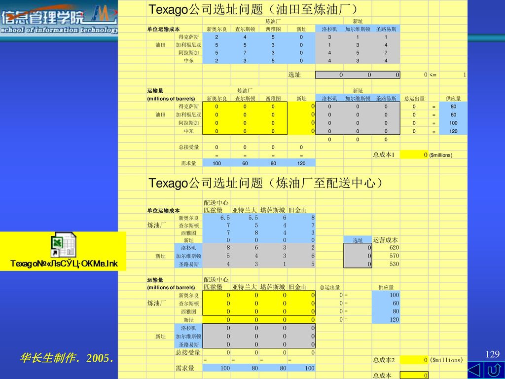
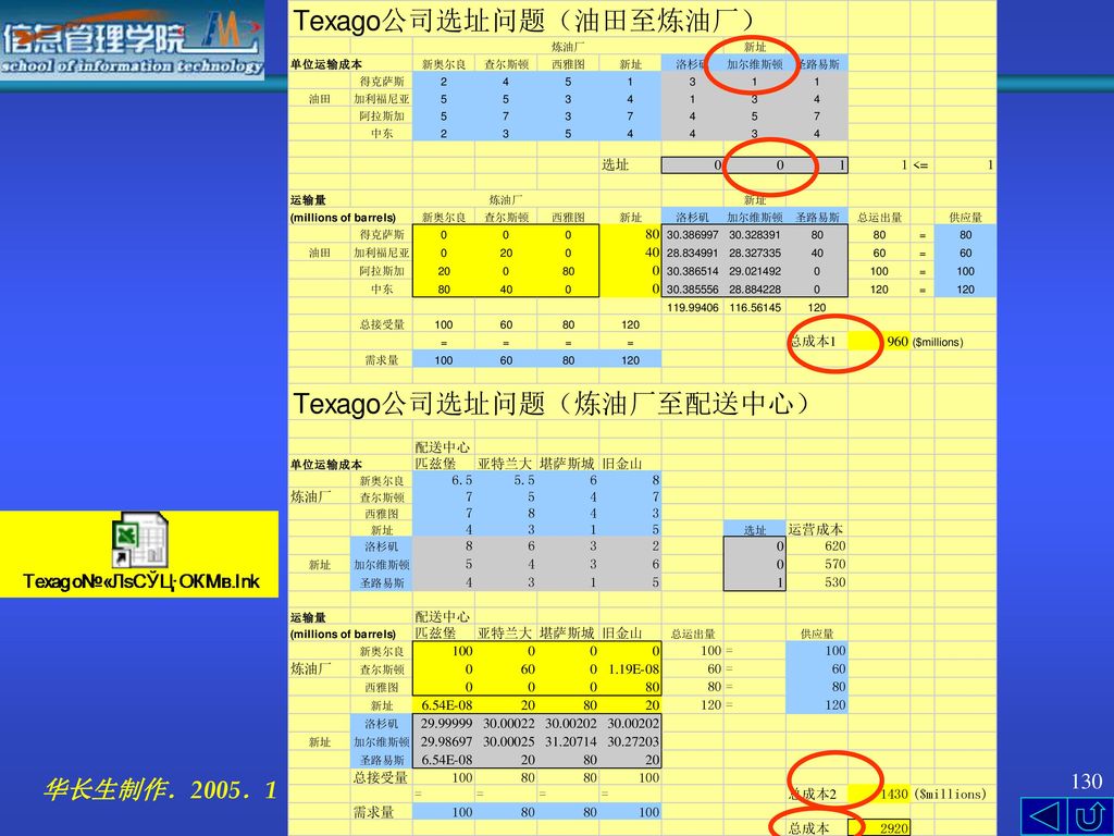
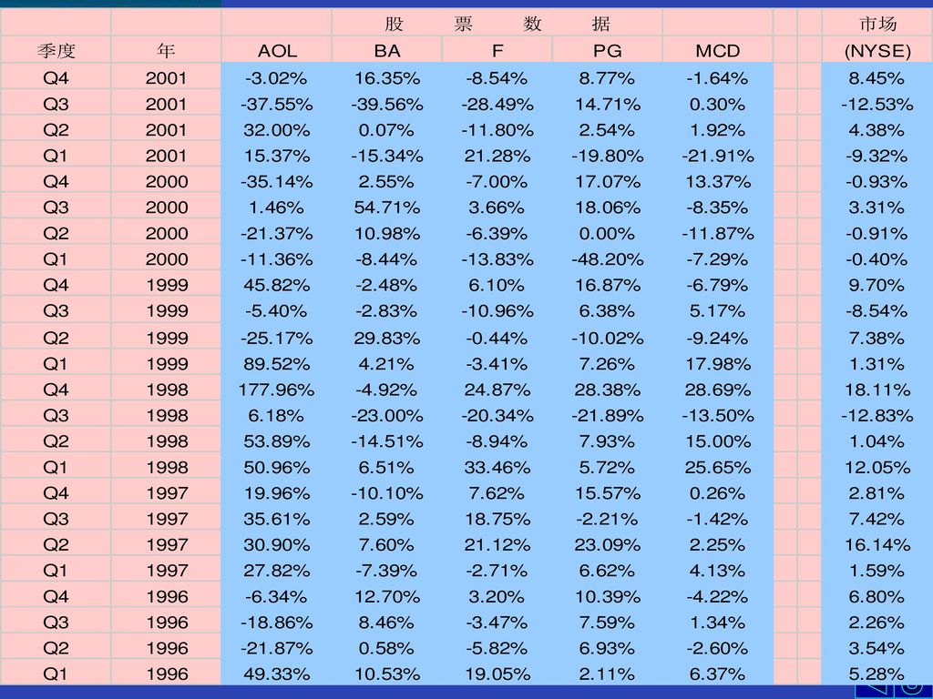
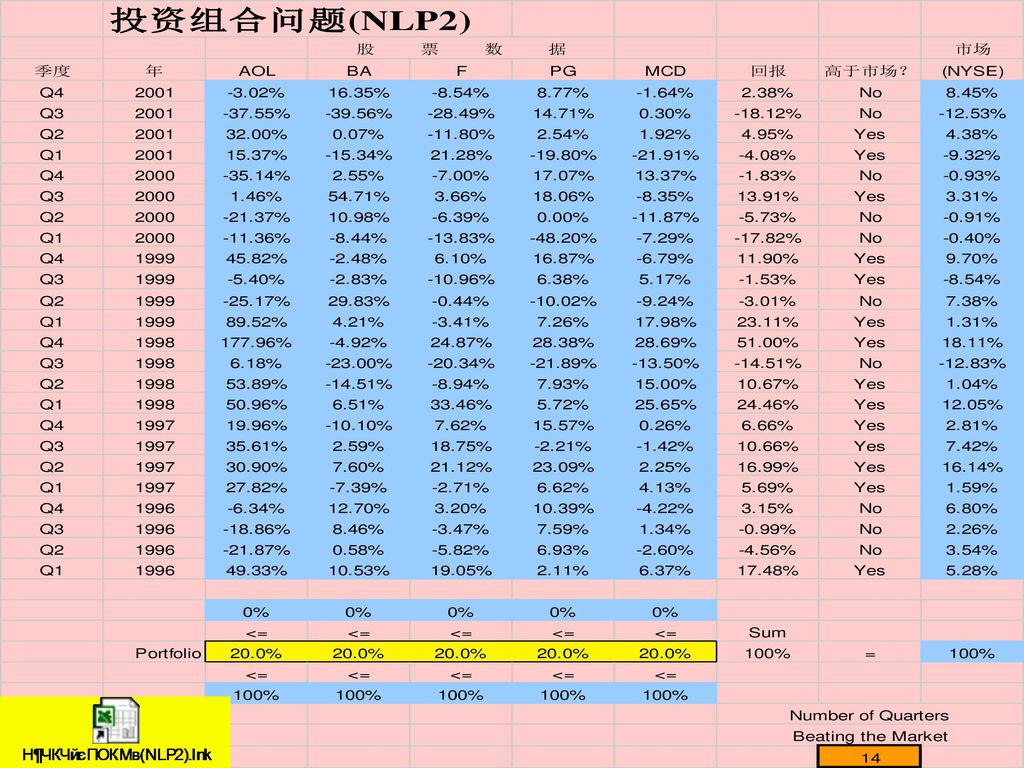

>")


>")


>")
