Zetasizer Nano 系列: 培训课程

Presentation on theme: "Zetasizer Nano 系列: 培训课程"— Presentation transcript:

1 Zetasizer Nano 系列: 培训课程
马尔文技术支持热线

2 Who Are Malvern Instruments?
马尔文仪器是一家英国公司，专注于设计和制造精确的测量仪器，应用于 粒子尺寸及其分布 粒子的电荷 分子量 粒子形态 分散体系的流体力学性质 在具体谈论仪器前，我想先简单介绍一下马尔文公司 Malvern Instrument is a company oriented in UK, whcih offers innovative solutions in material charachterization. We focus on ….. History of Malvern???

3 Zetasizer Nano 能够测量什么参数？
三种测量技术 动态光散射（Dynamic Light Scattering） 通过非侵入背散射 (NIBS)测量粒径及其分布 激光多普勒电泳（Laser Doppler Electrophoresis） 通过激光多普勒测速和相位分析光散射技术相结合的马尔文M3-PALS专利技术测量zeta电位 静态光散射（static light scattering) 分子量以及第二维利系数A2测量 在马尔文nano中我们主要使用了三种光散射技术

4 Zetasizer Nano系列: 粒子尺寸 Zeta电位 分子量 胶体颗粒，乳液，高分子溶液…… 高灵敏度 高浓度 维护简单
高灵敏度，准确率 高分辨率 分子量 蛋白质和高分子 Zetasizer 粒径范围 (nm) Zeta 电位测量的尺寸范围 (nm) 分子量范围 (Da) 0.6 to 6000 - 1000 to 2 x 107 5 to 10,000 1 to 3000 10000 to 2 x 107 我们可以由仪器上的标签来分辨Nano系列中不同的仪器配置。 Nano-s仅有动态和静态光散射装置。散射光的测量角度为173 度。测量范围为，对粒径范围。。。对分子量。。。 -z中仅配置了zeta电位测量装置。 Nano zs中结合了动静态光散射装置。 Nano s90中，仅配置了动静态光散射装置，散射光的测量角度为90度

5 Contents 动态光散射（第一天） 静态光散射及分子量的测定（第二天） Zeta 电位 测量原理（第二天） 测量原理
Nano系列的优化测量位置 由相关曲线得到粒径信息 – 预算法则 样品要求 样品制备 数据解释 静态光散射及分子量的测定（第二天） Zeta 电位 测量原理（第二天）

6 动态光散射 Dynamic Light Scattering
测试原理 Measurement Principle

7 Zetasizer Nano是如何测试粒子的粒径的?
动态光散射Dynamic Light Scattering (DLS)，也称光子相关光谱Photon Correlation Spectroscopy (PCS) ，准弹性光散射quasi-elastic scattering，测量光强的波动随时间的变化 粒子的布朗运动Brownian motion导致光强的波动 光子相关器correlator将光强的波动转化为相关方程 相关方程检测光强波动的的速度，从而我们得到粒子的扩散速度信息和粒子的粒径d(h) 从相关方程我们还可以得到尺寸的分布信息 DLS also named as pcs, quasi-elastic light scattering is to measure the fluctuation of the light scattering caused by the Brownian motion of the particles. From DLS we get the dynamic properties of the solute particles known as Brownian motion. The dynamic information of the particles is derived from an autocorrelation of the intensity trace recorded during the experiment.

8 Nano 的光学构造

9 动态光散射及布朗运动 微小粒子在悬浮溶液中的随意运动 布朗运动的速度依赖于 离子的大小 媒体的粘度

10 动态光散射 动态光散射测量依赖于时间的散射光强波动。由动态光散射可以得到粒子扩散速度的信息, 进而从Stokes-Einstein方程得到流体力学半径 hydrodynamic diameter (DH) k ： 波尔兹曼常数, T ： 绝对温度,  ： 粘度 kT 3DH D =

11 散射光强的波动 散射光强依赖于粒子的大小 散射光强的信息被传输到光子相关器
相关器连续加和处理从光散射信号中得到的很短时间的波动信息进而得到相关曲线 Time (s) Intensity (kcps) Small Particles Large Particles

12 相关方程表示随时间变化的相关性质 Time g2 1  = 0 Time 1 Time g2  = 1 Time Time 1 2 g2
Intensity Time g2 1  = 0 Time 1 Time g2 Intensity  = 1 Time Time 1 2 g2 Intensity 在起始时刻，光强乘以其自身，相关性能最好，定义为一 随着时间变化，光强的相关性越来越差，最后在无限长时刻，相关性为0  = 2 Time Time Intensity Time 1  2 3 g2  = 

13 相关方程（曲线） 初始斜率依赖于粒子大小 衰减的过程与粒子尺寸的分布相关 基线是否归零告诉我们是否有灰尘的存在 截距
This slide shows a schematic of a correlogram and illustrates the type of information that can be gained. Firstly, the time when the correlation starts to significantly decay indicates the mean size of the sample. Secondly, the gradient of the decay indicates the polydispersity of the sample. The steeper the gradient more monodisperse the sample is. Conversely, the more extended the decay becomes, the greater the sample polydispersity. Thirdly, the baseline of the correlation function gives information about the presence of large particles and or aggregates in the sample. The extrapolation of the data to zero time results in an intercept on the Y axis. This is the signal to noise ratio of the measurement. In the example shown in this slide, the intercept value is approximately zero point seven six. That is, the signal to noise ratio is zero point seven six for this measurement. As discussed earlier, a perfect signal would give an intercept value of 1. This is not possible during a real measurement as there is inherently a certain amount of noise present which reduces the intercept value obtained. The various reasons for the reduction in the intercept will discussed in more detail in future modules. 基线是否归零告诉我们是否有灰尘的存在

14 光强波动，相关函数和粒径分布 Small Particles Large Particles Apply Algorithm
Correlate Apply Algorithm Time (s) Intensity (kcps) Small Particles Correlate Apply Algorithm Time (s) Intensity (kcps) Large Particles

15 STOKES-EINSTEIN EQUATION
D 为扩散系数 d(h) 为流体力学直径 kB 为波尔兹曼常数 T 为绝对温度 h 为粘度 这里 我们通过。。。。。方程将粒子的运动速度和尺寸联系起来 2

16 动态光散射实际测量的是什么? 流体力学直径 流体力学直径

17 动态光散射实际测量的是什么? 流体力学直径 表面上枝接的一层分子将会降低扩散速度 因此，流体力学直径将会受到表面结构的影响 测得的直径

18 离子强度的影响 1/K, Debye 长度是带电颗粒双电层的厚度, 他取决于介质中的离子浓度 流体动力学直径
在较低离子强度 (如蒸馏水中)双电层是展开的 在较高离子强度(如高于10mM 盐溶液) 双电层是压缩的 流体动力学直径

19 动态光散射的特点： 上亿个粒子的统计学效果，使得对粒径及其分布的测量更加准确 对微量存在的大颗粒极其敏感 在溶液状态下测量颗粒的尺寸
测试速度快，所需样品少 需要溶液的粘度和折光指数等光学参数 所得到的尺寸分布正比于不同种类颗粒对光强的贡献率

20 所需参数 平均粒径和宽度 （分散系数） 粒径的体积和数量分布 温度 溶剂的粘度和折光指数（温度依赖性） 米氏理论需要: 样品的折光指数
样品的吸收率

21 动态光散射 由相关曲线得到粒径信息 : 运算法则

22 STOKES-EINSTEIN EQUATION
相关曲线 对于单分散体系 这里: G = Dq2 为衰减率 D 为扩散系数 q = (4 p n / lo) sin (q/2) 为散射矢量 n 为折光指数 lo 为照射光波长 q 为散射角度 STOKES-EINSTEIN EQUATION 对于但分散体系，通过单一指数方城

23 相关曲线 对于多分散体系 累积距法：得到平均粒子尺寸和分布系数（PD.I） 多指数分析模型：得到粒子实际尺寸和分布
这里我们利用。。法和。。法来拟和相关方程 累计距法 我们使用一个单指数多项是来拟和方程， 多指数模型我们使用一个多指数加和的模型来拟和方程 这里g1(t)是相关曲线中所有指数衰减的总和

24 累积距法 ISO13321 (1996)定义了应用于动态光散射技术的累积距法
这种方法给出了平均粒子尺寸 (z-average)和一个粒子的分布系数 (polydispersity index) 这个分析方法只需要分散剂的折光指数和粘度

25 累积距法 ISO13321 阐述用三次方多项式拟和相关方程 Ln[G1] = a + bt + ct2 b α z-均 扩散系数
2c/b2 为分布系数

26 z-均 直径 z-均直径(ZD)的定义: 累积距法得到的粒子平均尺寸对应于不同尺寸粒子散射光强的贡献 这里“平均”的概念特指用于光散射试验中
这种算法得到的平均尺寸对于大的缔合物及灰尘非常敏感

27 分布系数 分布系数定义 (PDI): 有累积距法得到的分布系数是一个无纲量的值，代表粒子尺寸的分布宽度
在Zetasizer Nano软件中他的范围是 0到1 如果PDI大于1，这说明样品的尺寸分布非常宽，可能不适合用动态光散射的方法来测量

28 分布系数 分布系数值 Comments <0.05 <0.08 0.08 to 0.7 >0.7
单分散体系，如一些乳液的标样。 <0.08 近单分散体系，但动态光散射只能用一个单指数衰减的方法来分析，不能提供更高的分辨率。 0.08 to 0.7 适中分散度的体系。运算法则的最佳适用范围。 >0.7 尺寸分布非常宽的体系。

29 对于分布的分析 对于相同的光散射数据，可以有几种不同的分析结果 为了适应不同的样品类型,两种NNLS 分析模型被应用到一起的软件中
General Purpose Multiple Narrow Modes 这两种算法的差异在于所得到的分布曲线的平滑程度 general purpose 算法适用于大部分分布状况未知的样品 multiple narrow mode 算法适用于分布状况不连续的样品

30 Zetasizer Nano 软件中的尺寸分布分析
由DLS而得的基本的尺寸分布，是一个根据光强的贡献率，并使用 (NNLS) 分析方法得到的分布 尺寸分布被表示为一个散射光相对光强对于对应的粒子尺寸的曲线 默认地，在尺寸分布中最多可以出现70个等级 The primary size distribution obtained from a dynamic light scattering measurement is the intensity-weighted distribution obtained from the chosen non-negative least squares analysis. This size distribution is displayed as a plot of the relative intensity of light scattered by particles (on the Y axis) versus various size classes (on the X axis). By default, there are 70 size classes which are logarithmically spaced.

31 Zetasizer Nano 软件中的尺寸分布分析
Here is an example of an intensity size distribution obtained from a dynamic light scattering measurement. The table shows the 70 size classes which are logarithmically spaced between a lower limit of zero point four nanometres and an upper limit of 10 microns on the X axis. The Y axis consists of the relative percentage of light scattered by particles in each of the size classes. The plot at the top right of the slide is the graphical representation of this data as a histogram. By default, the distribution is displayed as a frequency curve in the Nano software. An example is shown in the bottom right of the slide. There are various size distributions available in the Zetasizer Nano software and we will now look at each one in more detail.

32 光强粒度分布 体积粒度分布 数量粒度分布 从动态光散射得到最初的结果 结果基于粒子的散射光强度 对于大的粒子和灰尘十分敏感
分析样品的特性仅仅需要媒体的粘度和折光指数 体积粒度分布 使用光强分布数据应用Mie theory演算而来 等同于质量粒度分布 换算过程需要粒子的光学性质 粒子的折光指数 粒子对光的吸收率 The number size distribution is also derived from the intensity size distribution using Mie theory and the optical properties of the particles are also required to make this transformation. 数量粒度分布 使用光强分布数据应用Mie theory演算而来 换算过程需要粒子的光学性质 粒子的折光指数 粒子对光的吸收率

33 动态光散射 DLS 的粒子尺度分布 光强分布，体积分布和数量分布之间的相互转换基于以下前提:
所有的粒子都是球型的 所有的粒子都是均匀的，且密度相同 光学性质已知（折光指数，吸收率） 动态光散射 DLS 技术往往高估分布峰的宽度，这个影响可以从体积分布和数量分布的相互转换过程中体现 体积和数量分布中，峰的平均值和分布宽度只能用来估计成分的相对量。 While the transformation of the measured intensity distribution to volume or number seems straightforward, DLS users are strongly cautioned to be careful not to over analyse the results. Transformation from intensity to volume or number makes the following assumptions: (pause) all particles are spherical (pause) all particles have an homogenous and equivalent density (pause) the optical properties are known – that is the particle refractive index and absorbance and (pause) there is no error in the intensity distribution. The DLS technique tends to overestimate the width of the peaks in the distribution and this effect is magnified in the transformations to volume and number. The volume and number size distributions should only be used for estimating the relative amounts of material in separate peaks as the means and particularly the widths are less reliable. This will be illustrated with an example later in this module.

34 动态光散射 DLS 的粒子尺度分布 如果光强分布是一个相对平滑的峰，那么光强分布和转化得到的体积分布以及数量分布将会比较相似
如果光强分布中有一条非常明显的尾巴，或是多于一个分布峰，那么转化得到的体积和数量分布将会非常不同，并且会更真实地展现尾巴和其它峰 总的来说 d(intensity) > d(volume) > d(number) Let us go on to discuss the relationship between the intensity, volume and number size distributions. If the intensity distribution is a fairly smooth peak, conversion into volume will give a very similar distribution. If the intensity plot shows a substantial tail, or more than one peak, then the volume distribution will be quite different and give a more realistic view of the importance of the tail or second peak. In general the intensity distribution will always be larger than the volume distribution which, in turn, will be larger than the number distribution.

35 光强, 体积和数量分布 设想一个由相等数量的 5 nm 和 50nm 球型粒子组成的混合物
体积分布 光强分布 (Rayleigh Theory) N1*3/4πr13 : N2*3/4πr23 N1V1:N2V2 N1:N2 N1V12 : N2V22 Relative % in class Diameter (nm) 5 50 1 Relative % in class Diameter (nm) 5 50 1 1,000 Relative % in class Diameter (nm) 5 50 1,000,000 1 为了更好的理解光强分布，我们看一下下面的例子 我们的软件中可以同时提供这三种分布的信息 数量平均粒径  28nm 体积平均粒径  49nm 光强平均粒径 = 50nm

36 光强，体积和数量分布: 例子 60nm 和 220nm 聚苯乙烯乳液标样1:1 体积混合 z-均直径 = 168nm PDI = 0.215
Peak 1 Peak 2 Mean (nm) % Intensity 231 86.3 65.8 13.7 Volume 232 50.3 61.8 49.7 Number 184 2.6 58.2 97.4 To illustrate the relationship between intensity, volume and number size distributions, here is an example of a mixture of different sized polystyrene latex standards. These latex standards were mixed in equal volumes. This record is contained in the example results file which is provided with the Zetasizer Nano software. The z-average diameter obtained was one hundred and sixty eight nanometres with a polydispersity index value of zero point two one five. If we first look at the intensity size distribution, we find that the main peak has a mean diameter of two hundred and thirty one nanometres. This peak constitutes around 86 percent of the distribution. This is because the larger particles in the sample are scattering more light compared to the smaller population When the distribution is viewed in volume, the percentage of each peaks is approximately 50%, which corresponds with the ratio at which the 2 latex standards were mixed at. When the result is viewed in number, the vast majority of the distribution is contained in the smaller sized peak. So if this sample was viewed under an electron microscope, the smaller particles would be dominant. That is, on a number basis, the sample appears to consist mainly of the smaller population of particles. The intensity distribution however, detects the presence of larger particles which may be missed by a number based technique.

37 体积和数量分布: 建议 建议在报告个分布峰所对应的尺寸时，使用光强分布曲线的结果 在报告各个峰的相对数量时，使用体积或者是数量分布 Peak
As we have discussed in a previous slide, DLS tends to overestimate the width of the peaks in the distribution and this will become even more significant upon transformation into volume or number. In addition, we have seen that a small amount of large particles present in the sample will dominate the intensity size distribution obtained from a DLS measurement. Therefore, it is recommended to use the intensity size distribution for reporting the size of each mode in the distribution but to the use volume or number data for reporting the relative amounts of each particle family in the sample. This recommendation can be highlighted with the example shown here. The intensity and volume particle size distributions shown in this slide were derived from a 2 to 1 volume mixture of 60 and 220nm polystyrene latex standards. The intensity particle size distribution shows a bimodal with peak means of 59 and 220 nanometres respectively. The relative percentages of each mode based upon the intensity data are 21 and 79 percent respectively with the larger peak being due to the larger sized population. However, conversion to volume gives relative percentages of 67 and 33 percent respectively. Therefore, the recommended way of reporting this result is to use the peak mean diameters from the intensity size distribution together with the relative percentage values obtained from the volume distribution. Peak DI (nm) % Int % Wt 1 59 21 67 2 220 79 33

38 动态光散射 Dynamic Light Scattering
Nano 系列中的优化测量位置

39 Nano 的光路系统

40 非侵入背侧光散射特点 (Non Invasive Back Scatter (NIBS) Overview)
在Nano S 和 Nano ZS 系列中，光散射检测角度为173o ，因此成为背光散射 光学系统不穿过样品，因此称为非侵入性 NIBS所观察到的样品散射体积为在90o （ Zetasizer Nano S90 ）条件下的8倍，因此能够得到更多的散射光强，仪器也更加灵敏 更高的灵敏度使仪器能够检测低浓度下小尺寸的粒子 激光不需要穿过整个样品，因此降低了多次光散射效应。可以检测较高浓度的样品 多次光散射效应通常降低粒子的表观尺寸，增加光子相干曲线的截距 污染物，如灰尘粒子，得散射光通常在较小的角度有比较大的散射光强 因此背侧光散射可有效的降低灰尘的影响 多次光散射是指对于一些高浓度样品我们检测到的散射光经过多个粒子的多次连续散射

41 NIBS: 可调整检测位置 小粒子/ 稀溶液 高浓度溶液 减小散射光体积 较大的散射提体积 降低多次散射影响 检测器 激光 凸透镜 样品池
 检测器 激光 凸透镜 样品池 高浓度溶液 减小散射光体积 降低多次散射影响

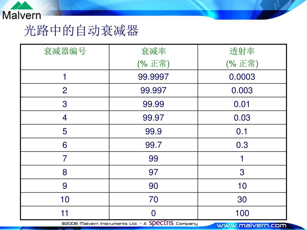
42 光路中的自动衰减器 自动衰减器起到调整光学强度的作用，使得粒子的散射光在一个仪器可以检测的范围之内
Zetasizer Nano自动水衰减器有11个光学衰减镜片涵盖100% 到 % 的透射率 透射率指到达样品的激光的强度占光源激光强度的百分比 在测量粒子大小的过程中，自动衰减器会自动调节透射光的强度，直到检测器检测到的光强小于 500kcps

43 光路中的自动衰减器 衰减器编号 衰减率 (% 正常) 透射率 1 99.9997 0.0003 2 99.997 0.003 3 99.99
0.01 4 99.97 0.03 5 99.9 0.1 6 99.7 0.3 7 99 8 97 9 90 10 70 30 11 100

44 测试时间 测试时间由样品的散射光强度决定 散射光越弱测试的时间越长 每个测试都被分成一系列10秒钟的子测试以减少灰尘对测试的影响
仪器默认 50% 的平均光强最小的子测试为有效测试，被用来进行数据分析

45 动态光散射 Dynamic Light Scattering
样品要求

46 International Standard ISO 13321 (1996)
样品要求 样品应该较好的分散在液体媒体中 理想条件下，分散剂应具备以下条件: 透明 和溶质粒子有不同的折光指数 应和溶质粒子相匹配 (也就是：不会导致溶胀, 解析或者缔合 掌握准确的折光指数和粘度，误差小于0.5% 干净且可以被过滤 International Standard ISO (1996) Let’s begin by discussing the sample requirements. The sample should consist of well-dispersed particles in a liquid medium. Ideally, the dispersant should meet the following requirements: It should be transparent. It should have a different refractive index from the particles. It should be compatible with the particles (i.e. not cause swelling, dissolution or aggregation). Its refractive index and viscosity should be known with an accuracy better than 0.5%. It should be clean and filterable. These recommendations are made in the International Standard on dynamic light scattering I S O one three three two one.

47 动态光散射对粒子尺寸的下限 依赖于： 粒子相对于溶剂产生的剩余光散射强度 仪器敏感度
折光指数 样品浓度 仪器敏感度 激光强度和波长 检测器敏感度 仪器的光学构造 We now discuss what the lower and upper size limits of dynamic light scattering are. We start with the lower size limit of the technique. It is dependent upon the amount of excess scattered light the particles generate compared to the suspending medium and on the sensitivity of the instrument. The excess scattering generated will depend on the relative refractive index and sample concentration. The relative refractive index is the particle refractive index compared to the dispersant refractive index. The sensitivity of the instrument will be governed by the laser power and wavelength, the sensitivity of the detector and optical configuration of the system. A backscatter instrument such as the Nano S will be able to measure smaller particles more easily than a conventional 90 degree instrument such as the Nano S90. The lower size limit is typically 2nm

48 动态光散射对粒子尺寸的上限 DLS 测量粒子无规则的热运动/ 布朗运动 （Brownian motion ）
若粒子不进行无规则运动，则仪器无法应用 粒子尺寸的上限定义于沉淀行为的开始 因此上限取决于样品 – 应考虑粒子和分散剂的密度 使用更高粘度的分散剂去阻止或者降低粒子的沉淀速度没有任何优势，因为布朗运动的速度将会被等同的降低 We move on to discuss what the upper size limit of the technique is. Dynamic light scattering measures the random motion of particles undergoing Brownian motion and the technique will not be applicable when the particle motion is not random. Therefore, the upper size limit is normally defined by the onset of particle sedimentation and is sample dependent. Both the particle and dispersant density have to be considered. For example, a uranium colloid with a density approximately equal to 19 may have an upper size limit of only 50nm, whereas for a liposome, whose density is virtually the same as water, this upper limit may be up to 5 microns. There is no advantage in suspending a material in a more viscous medium to try to reduce or prevent sedimentation. The benefit of doing this is offset by the fact that Brownian motion is reduced by exactly the same amount.

49 样品浓度总结 从动态光散射得到的样品尺寸应该不依赖于浓度 (ISO 13321) 每种样品都有其理想的测试浓度范围
如果浓度太低，可能散射光强不足以进行试验 这种状况不太可能出现在Nano S/Nano ZS系列中，除非在一些极端条件下 如果样品浓度太高，实验结果可能会依赖于浓度 为了得到正确的尺寸信息，可能会需要在不同的浓度下检测样品尺寸 We now move on to discuss the lower and upper concentration limits of dynamic light scattering. The result obtained from a DLS measurement should be independent of sample concentration – this is highlighted in I S O one three three two one. Each type of sample material has its own ideal range of concentration where measurements should be made. If the concentration is too low, there may not be enough light scattered to make a measurement. This is unlikely in the Nano S/Nano ZS except in extreme circumstances. If the concentration is too high, the result may not be independent of sample concentration. During method development, determining the correct sample concentration may involve several size measurements at different concentrations.

50 样品浓度下限 依赖于： 粒子相对于溶剂产生的剩余光散射强度 仪器敏感度
折光指数 样品浓度 仪器敏感度 激光强度和波长 检测器敏感度 仪器的光学构造 Let us begin by looking at the lower concentration limit of dynamic light scattering. The factors influencing the lower concentration limit of the technique are the same as for the lower size limit. They are the amount of excess scattered light the particles generate compared to the suspending medium and the sensitivity of the instrument. A backscatter instrument such as the Nano S will be able to measure lower sample concentrations than a conventional 90 degree instrument such as the Nano S90 due to the increased sensitivity associated with backscatter detection. The lower size limit is typically 2nm

51 样品浓度上限 对于高浓度样品，由动态光散射测得的表观尺寸可能会受到不同因素的影响 多重光散射 – 检测到的散射光经过多个粒子散射
扩散受限 – 其他粒子的存在使得自由扩散受到限制 聚集效应 – 依赖于浓度的聚集效应 应电力作用 – 带电粒子的双电层相互重叠，因而粒子间有不可忽视的相互作用。这种相互作用将影响平移扩散 At high sample concentrations, the apparent size reported from a dynamic light scattering measurement may be influenced by various factors. Firstly, there could be multiple scattering effects. This is where light scattered from diffusing particles is re-scattered by other particles. Secondly, there may be restricted diffusion. This is where the presence of other particles blocks or hinders free particle diffusion. Thirdly, aggregation effects might be present where there is a concentration dependent aggregation of primary particles. Finally, there may be electrostatic interactions occurring. This is where overlapping electric fields lead to soft particle interactions that can influence the translational diffusion.

52 样品浓度上限 表观 z-Average 直径 (nm) 样品浓度 低 高 可测量浓度 多次光散射 Nano S 可测量浓度
When multiple scattering is insignificant the size will be independent of concentration. The plot shown in this slide illustrates the effect of sample concentration on the mean diameter obtained for both a 90 degree and backscatter instrument. In both instruments, the size obtained is independent of concentration when the sample concentration is low. However, as the concentration of the sample is increased, the presence of multiple scattering will begin to influence the size obtained. In a backscatter instrument such as the Nano S, the concentration over which the sample can be measured correctly is greatly extended compared to the 90 degree system due to the reduction of multiple scattering effects. Instruments which have backscatter detection extend the concentration over which samples can be measured before seeing the effect of multiple scattering. Nano S90 低 高 样品浓度

53 二氧化硅浆料的粒径以及分散系数随浓度的变化
样品浓度上限 二氧化硅浆料的粒径以及分散系数随浓度的变化 When multiple scattering is insignificant the size will be independent of concentration. The plot shown in this slide illustrates the effect of sample concentration on the mean diameter obtained for both a 90 degree and backscatter instrument. In both instruments, the size obtained is independent of concentration when the sample concentration is low. However, as the concentration of the sample is increased, the presence of multiple scattering will begin to influence the size obtained. In a backscatter instrument such as the Nano S, the concentration over which the sample can be measured correctly is greatly extended compared to the 90 degree system due to the reduction of multiple scattering effects. Instruments which have backscatter detection extend the concentration over which samples can be measured before seeing the effect of multiple scattering.

54 推荐样品浓度 粒子尺寸 最小推荐浓度 最大推荐浓度 Nano S90/ZS90 Nano S/ZS < 10nm 5mg/ml
Only limited by the sample material interaction (gelation, aggregation) 10nm to 100nm 1mg/ml 0.1mg/ml 0.1% w/v 5% w/v (assuming a density of 1gcm-3) 100nm to 1μm 0.01mg/ml 0.01% w/v 1% w/v (assuming a density of 1gcm-3) > 1μm An important factor in determining the maximum and minimum concentrations the sample can be measured at is the size of the particles. This table is an approximate guide for obtaining results which are independent of concentration for samples with a density near to 1 gramme per cubic centimetre. If such concentrations cannot be selected easily, it is recommended that various concentrations of the sample should be measured in order to determine if concentration dependent effects such as particle-particle interactions or multiple scattering, are present.

55 动态光散射 Dynamic Light Scattering
样品池装载，样品制备和仪器校准

56 注入溶液 只用干净的样品池！ 缓慢注入溶液以避免气泡 如果使用注射管滤膜过滤样品，请放弃开始的几滴溶液以避免在滤膜下面的灰尘进入样品池
使用滴液管，同时倾斜样品池 如果使用注射管滤膜过滤样品，请放弃开始的几滴溶液以避免在滤膜下面的灰尘进入样品池 用盖子将样品池封住 Now we discuss the filling of a sizing cell. When filling the cell, there are several actions to consider. It is recommended that only clean cells should be used and all size cells should be rinsed or cleaned with filtered dispersant. The cell should be filled slowly to avoid air bubbles. Using a pipette and tilting the cell at an angle will aid with this. If using syringe filters for the dispersant, discard the first few drops in case of any residual dust particles in the filter that may contaminate the dispersant. A minimum sample volume must be provided in the cell for successful measurements to be made. This minimum volume depends upon the actual cell type and it is easier to ensure a certain depth of the sample in the cell. This minimum is 10 millimetres from the bottom of the cell. The measurement is made 8 millimetres from the bottom of the cuvette. It is recommended that the maximum level should be no more than 15 millimetres from the bottom of the cell. This is to minimise thermal gradients within the sample which will reduce the accuracy of the temperature control. The level of the sample in the cuvette can be checked against the figure on the inside of cell area lid. Finally, when the cell has been filled with the sample, it is advisable to cap the cell to avoid dust contaminating the sample.

57 将样品池放入仪器 The size cell is inserted into the instrument by firstly pushing the button on the front to open the cell area lid. Secondly, the cell is pushed into the cell holder until it stops. The orientation of the cell in the instrument is very important as some cells have opaque surfaces as well as polished optical surfaces. A polished optical surface must be facing the front of the instrument. The polystyrene disposable cells have a small triangle at the top to indicate the side that should face the front of the instrument. If a flow cell is used, insert the sample tubes into the threaded inserts and screw into the top of the flow cell and then push both tubes down into the pinch valve on the side of the cell area. Thirdly, place the thermal cap over the cell. Do not fit it if you are using the flow cell. Fourthly, close the cell area lid. It is worth noting here that some cells, particularly the glass and quartz ones, can feel quite tight when being inserted into the cell area. It is important that the cell is inserted all of the way into the cell holder. To ensure that this is the case, press firmly down on the top of the cell.

58 样品制备: 稀释 如果样品浓度很高，则需要将溶液稀释
稀释样品时须注意保证保持样品原来的性质，如吸附在粒子表面的物质和原溶液之间的化学/物理平衡 稀释溶液应和原来的样品溶液保持相同的性质 如果样品很多，稀释液可以由过滤或者离心原来的样品溶液除去溶质而得到 如果样品很少，稀释液应尽量按原溶液性质制备 We now move on to discuss some important points in the preparation of samples for successful dynamic light scattering measurements. If the sample is too concentrated, it will need to be diluted. Dilution needs to be carefully performed to ensure that the equilibrium of any absorbed species between the particle surface and bulk solution is preserved. The diluent should be the same as the continuous phase of the original sample. The diluent could be obtained by filtering or centrifuging the original sample and obtaining a clear supernatant suitable for dilution. If this is not possible, the continuous phase should be made up to be as close as possible to that of the sample.

59 样品制备: 过滤 灰尘是光散射实验最主要的问题之一，灰尘的存在可能导致测试失败 为了避免灰尘的影响，样品溶液在测试之前应该被适当的过滤
商业化的注射管过滤膜网眼的尺寸通常从 1μm 到 20nm Dust is one of the major problems in DLS measurements and may bias the results obtained. To avoid any possible dust contamination during dilution, the medium should be ideally filtered. Commercial syringe filters are available for use with pore sizes ranging from 1 micron down to 20 nanometres.

60 校准和检查 动态光散射Dynamic light scattering是一种绝对测试，因此不需要校准
然而光学仪器如光路，有时会因环境（如温度，外力）改变而改变，应当定时检查 检查的频率以用户的使用方式和需求而定 检查可由检测标样（聚苯乙烯乳液）来完成 马尔文公司推荐Duke Scientific Corporation ( 的聚苯乙烯乳液为标准样品 标准起源于 NIST – the National Institute of Standards and Technology ( Read slide

61 动态光散射 数据处理 Zetasizer Nano 系列

62 数据处理 实验得到的原始数据对于之后的计算分布的运算过程非常重要 原始数据的质量越好，所得结果的重复性越好
为了有助于更好的解释实验数据，马尔文建议观看不同的报告页，并将实验参数加入DTS软件中的默认选项中，显示在报告中

63 数据解释 报告 专家建议报告（Expert Advice Report） 尺寸质量报告（Size Quality Report）
相关曲线报告（Correlogram Report） 累积距拟和报告（Cumulants Fit Report） 多指数拟和报告（Multimodal Fit Report） 参数 平均光强（Mean Count Rate） 截距（Measured Intercept） 检测位置（Measurement position） 累积距拟和误差（Cumulants fit error） 多指数拟和误差（Multimodal fit error） 衰减率（Attenuator） 原始光强（Derived Count Rate）

64 光强的重复性 同一个样品重复至少三次测试-光强误差应该在百分之几之内 在连续测试过程中光强增强意味着: 在连续测试过程中光强减弱意味着:
粒子聚集 在连续测试过程中光强减弱意味着: 粒子沉淀 粒子溶解 在连续测试过程中光强无规则变化意味着: 粒子不稳定 (聚集或分离)

65 z-均直径重复性 多次z-均直径的测试结果误差应在1%-2%之内 z-均直径增长意味着: z-均直径下降意味着: 粒子聚集
温度不稳定 (粘度随时间变化) z-均直径下降意味着: 粒子沉淀 粒子溶解 温度不稳定(粘度随时间变化)

66 数据分析: 相关曲线图 相关曲线图显示在特定时间段下每个通道得相干性，其中包含样品的信息 曲线的形状能够显示一些可能出现的明显的问题
应检查相关曲线中的噪音状况 噪音可由不同原因造成 - 光强太弱，样品不稳定，或者一些外部原因如散射光和其它杂散光源的相互干涉

67 数据分析: 相关曲线图 小粒子 中等分散指数 存在大的粒子/缔合 (基线不平)

68 数据分析: 相关曲线图 大粒子 高分散指数 很大的粒子/缔合物 (基线不平)
很大的粒子/缔合物 (基线不平) 截距 > (number fluctuations causing baseline definition problems)

69 数据分析: 相关曲线图 双峰分布 高分布指数 无大粒子/缔合物 (基线平)

70 数据分析: 相关曲线图（小颗粒） 提高早期信号信躁比（1-10 us） 提高后期信号信躁比（>100 us） 增加测试子测试数目
增加收集时间

71 累积距/分布拟和报告 累积距和分布拟和报告分别显示这两种拟和方法的质量，从中我们可以看出（1）z-均直径和分散度（2）光强分布是否可信
认为拟和误差小于0.005为较好结果

72 累积距/分布拟和报告 双分布样品的相关曲线和光强分布
尺寸质量报告给出的对于累积距法的拟和误差较大，说明测得的z-均直径 (301nm) 并不可靠

73 累积距/分布拟和报告 由于双分布累积距拟和的结果很不好，然而分布拟和的结果非常好
因此，尽管这个测试的z-均半径不可靠，但是光强尺寸分布是很准确地 Distribution fit Cumulants fit

74 尺寸分布的重复性 尺寸分布结果由 NNLS 方法分析而来，对于这些结果应该检查分布峰的位置和包含的面积的重复性
如果分布没有重复性，马尔文建议重新测量，并将测试时间延长

75 提取测试标准操作过程(SOP) DTS软件中具有提取任何结果SOP的功能，这是一个非常有利的工具，使得我们可以查看数据的质量
可以从测试的电脑中提取测试中的报错信息(例如：与样品类型不匹配的的测试位置，手动设置的超时测量时间

76 尺寸质量报告 对于任何选择的测试纪录，尺寸质量报告包含12个步检测步骤
如果任意一步检测的结果在一个特定的范围之外，一个警告信息和一个可能原因的建议将会出现 如果所有的检测都通过，会出现一条“Result Meets Quality Criteria” 信息

77 Contents 动态光散射 静态光散射及分子量的测定 测量原理 应用实例 Zeta 电位

78 静态光散射 Static light scattering (SLS)
在静态光散射中，我们检测溶质粒子的绝对散射光强虽浓度的变化 在Zetasizer Nano ZS中，我们在一个角度检测光强 通过Debye曲线我们可以测量 绝对分子量 第二维利系数

79 第二维利系数 2nd virial coefficient (A2)
一个热力学性质，形容溶质和溶剂间的相互作用 当 A2 > 0, 溶质分子稳定的存在于溶剂中 当 A2 = 0, 溶质分子和溶剂分子的相互作用等同于溶质分子内部相互作用被称为 theta 溶剂条件 当 A2<0, 溶质分子不能稳定存在于溶剂中，形成结晶或者聚集

80 什么样的样品适合静态光散射? YES NO Proteins Polymers Dendrimers Liposomes Emulsions
Mixtures NO

81 静态光散射 I  (MW2) (C) (Rayleigh Equation) K ：光学常数 C ：浓度 M：分子量 Rq ：样品的瑞利比
在静态光散射中，我们不考虑光的波动仅仅检测平均光强。 K ：光学常数 C ：浓度 M：分子量 Rq ：样品的瑞利比 A2：2nd 维利系数 P() ：形态因子

82 静态光散射 o = 激光波长 NA = 阿佛家德罗常数 no = 溶剂折光指数 Rg = 均方旋转半径
dn/dc = 折光指数对浓度的增量 Rg = 均方旋转半径  = 检测角度 IA = 绝对光强 (I样品 – I溶剂) no = 溶剂 IT = 标准物光强 (toluene) nT = 标准物 (toluene) 折光指数 RT = 标准物瑞利比 (toluene) 者是静态光散射检测方程。 对于小粒子，同场小于激光波长的1/10 p(o)约等于一，也就是说散射光强不再有角度依赖性

83 因此从KC/R 对浓度做曲线，截距值为分子量的倒数1/M，斜率为第二维利系数A2
静态光散射 对于瑞利散射, P() = 1 因此方程被简化 Debye 曲线 (y = mx + c) 如果我们已。。。对。。。作图 因此从KC/R 对浓度做曲线，截距值为分子量的倒数1/M，斜率为第二维利系数A2

84 样品制备 在适合的溶剂中，制备一系列已知准确浓度的样品样品溶液 具体浓度依赖于所测量的样品，一般在0.1-10g/L 溶剂 1 2 3 4

85 样品制备 所有使用的玻璃容器，吸液管，样品池，溶剂，均应无尘
用过滤膜过滤所有的溶剂，分散剂 (e.g. Whatman Anotop 20nm pore size filters)

86 分子量测定应用实例 (Lysozyme in PBS)
1/截距 = 14.6KDa 斜率 = x 10-4

87 Contents 动态光散射 静态光散射及分子量的测定 Zeta 电位 测量原理 样品制备 样品测试 测试中的选择 数据解释

88 Zeta电位 Zeta Potential 电泳光散射 Electrophoretic Light Scattering (ELS) 激光多普勒电泳 Laser Doppler Electrophoresis (LDE) 理论概述

89 胶粒分散体系（colloidal dispersion）的稳定性
胶粒分散体系的稳定性取决于粒子间短程吸引力（范德华力）和远程排斥力（静电力）之和 胶粒分散体系的可以通过不同机制失去稳定性 稳定体系 絮凝 凝聚 沉淀 相分离

90 静电力排斥（ELECTROSTATIC）
维持分散体系的稳定性 粒子稳定的存在于溶液中主要基于以下两种机制: 静电力排斥（ELECTROSTATIC） Easy to measure the controlling parameter (zeta potential) Reversible May only require change in pH or ion concentration （位阻效应）STERIC Simple, but limited options Irreversible An extra component

91 水溶液中表面电荷的产生 大部分水溶液中的胶体系统带一定量的电荷 电荷的产生机制有很多取决于粒子的材料和媒体的性质
表面基团的离子化 粒子表面有失去离子的趋势 离子的表面能够吸收离子或者粒子性表面活性剂 表面电荷导致在粒子周围抗衡离子浓度的增加

92 Zeta电位(Zeta Potential)
Slipping plane Zeta电位同时依赖于粒子表面和分散剂的化学性质 对于静电力稳定的分散体系，通常是Zeta电位越高，体系越稳定 体系稳定与否通常以Zeta电位是否大于 30mV为标准 Particle with negative surface charge 影响Zeta电位的因素 Stern layer 对于一个带点粒子，通常对电位由三个定义。由于粒子带点，在粒子的表面的电势称为表面zeta电势。在粒子表面有一层抗衡离子紧密地和表面结合在一起，这个边缘的电势称为stern电势，在外层还有一些离子和带电粒子松散的结合在一起，但是这层离子区别于溶剂中自由运动的离子,这一层电势称作zeta电势 Diffuse layer 影响Zeta电位的因素有： pH变化, 电导率 (浓度，盐的类型) 组成成分浓度的变化 (如高分子，表面活性剂) -100 - { Surface potential Stern potential mV Zeta potential Distance from particle surface

93 什么是Zeta电位? Zeta电位同时依赖于粒子表面和分散剂的化学性质 对于静电力稳定的分散体系，通常是Zeta电位越高，体系越稳定
体系稳定与否通常以Zeta电位是否大于 30mV为标准 Zeta电位是粒子间静电力相互作用的标尺，可以被用来预测分散体系的稳定性以及存储时间 The one idea to remember about zeta potential, is that it is not the same parameter as surface charge or surface potential. This difference may not be very important for simple systems such as a dispersed mineral oxide in demineralised water, but as soon as there are other components in the dispersion that interact with the surface. These components can change the magnitude of the zeta potential or even reverse the sign of the charge. The zeta potential is the value of the potential at a distance from the surface known as the slipping plane. This is the distance within which the ions move as part of the particle, and from the charge point of view defines the particle. Particles interact according to the magnitude of the zeta potential not their surface change.

94 测量 Zeta电位 电泳是在施加电场下，带电粒子相对于液体媒体的运动 带电粒子以特定的速度运动，运动的速度取决于: - +   电场强度
媒体的介电常数 媒体的粘度 Zeta电位 + -  

95 （ELECTROPHORETIC MOBILITY）
电泳 ZETA电势和电泳淌度相关UE （ELECTROPHORETIC MOBILITY） 根据HENRY方程 UE = 2 e z f(k a) 3 h z ：zeta电势 UE ：电泳淌度 e ：介电常数 H：粘度 f(k a) ： Henrys 方程

96 Henrys 方程 F(ka) 非极性溶剂 极性溶剂 Huckel 近似 F(ka) = 1.0 Smoluchowski 近似

97 Nano的光学构造 参考光不通过样品池 衰减镜片调整入射光的光强 这样仪器可以检测很宽浓度范围内的样品

98 激光多普勒电泳 Laser Doppler Electrophoresis
一束激光经过毛细管样品池中电场中的样品。样品在外加电场的作用下进行电泳运动，因此由运动粒子发出的散射光会有频率的移动 频率移动 f 等于:  ：粒子的速度  ：继光的波长 q ：散射角度 f = 2 sin(/2)/

99 用激光多普勒电泳测量Zeta电位 v F1 F1 F2 粒子速度 V=0 散射光与入射光有相同频率 粒子速度 V>0
散射光品率高于入射光 F2 F1

100 用激光多普勒电泳测量Zeta电位 因为光源的频率很高 (1014Hz), 频率的移动只能通过光学混拍来测得
这种技术是通过检测从一个光源分出的两束光程几乎相同的激光相干性 其中一束光必须通过样品体系(这束光被称为散射光) 另一束光 (称为参考光)不通过样品体系 散射光和参考光在检测器处相干，引起光强的波动

101 光强的波动是怎样被引发的? 参考光 F1 和散射光 F2 F1 F2 将两束光结合

102 相干的结果产生一个频率小得多的调制光源，这束光的频率等于参考光和散射光频率的差
光强的波动是怎样被引发的? 参考光 F1 和散射光 F2 F1 F2 A A 这两束光在A 相干加强， 在 B 相干减弱 B F1 - F2 = f 相干的结果产生一个频率小得多的调制光源，这束光的频率等于参考光和散射光频率的差

103 检测器检测的是光强随时间的波动，进而得到拍频
拍频被聚焦到检测器处 检测器检测的是光强随时间的波动，进而得到拍频

104 检测多普勒平移的方向 多普勒平移的方向由比较拍频的大小和一个参考频率的大小 参考频率由调制在参考光源光路上的一面反光镜生成
粒子在施加电场中的移动将会造成区别于调制频率的频率(320 Hz)的移动 这样我们得到zeta电位的明确的符号

105 高频电场转换 FFR (Fast field reversal)
电动力学理论分析显示当施加一个电场于一个毛细管样品池上，带电粒子达到最终速度所需的时间要比电渗建立起来的时间至少快一个数量级 如果施加电场的转换频率很高，例如50Hz, 我们就可以检测到带电粒子的速度，同时避免电渗的影响. 但是分辨率可能会偏低 正极 负极 使用高频转换的原因是要避免电渗的影响 高频电场转换中的电渗 Stationary Plane

106 混合模式测试-Mixed Mode Measurement (M3)
混合模式测试是一个专利方法，使得测试可以在毛细管中的任何一点进行 这个模式中包含高频电场反转 (FFR) 和低频电场反转 (SFR) FFR 测试了在电渗开始之前带电粒子真实的电泳运动速度 SFR 改善了测试的分辨率，提供电势分布的信息 相分析光散射Phase Analysis Light Scattering （PALS）被用于检测在FFR模式下粒子的移动性

107 M3 测试技术 高频电场转换1000Hz能够准确地测量zeta电位的平均值，但是分辨率较低
-50 mV -110 低频电场的转换可以给出更好的分辨率但是受到电渗的影响 This is the measurement from fast filed reversal By combining the fast mode and slow mode measurement, we get better resolution and also the speed of the electroosmotic flow 通过M3测试技术，结合高频和低频电场的转换，我们既得到准确地平均zeta电位，又得到了较高的分辨率

108 常规模式（General Purpose） 相曲线
FFR（高频电场转换） SFR（低频电场转换） 通过相分析和复利叶变换得到电位的分布 通过相分析得到平均电位 (Ep)

109 PALS only to obtain mean (Ep) – no distribution or width
单项模式 Monomodal 相曲线 FFR only PALS only to obtain mean (Ep) – no distribution or width

110 Zeta电位（Zeta Potential）
样品制备和仪器校正

111 zeta电位试验中的样品测试 Zeta电位测试中对样品的要求不像尺寸测试对样品的要求那样严格，样品可以看上去不很透明
可测浓度的上限依赖于粒子尺寸和光学性质 粒子的尺寸越大，需要样品的浓度越稀 粒子和分散剂的折光指数差越大，需要样品浓度越稀 当溶液需要稀释的时候，稀释的方式对于最终结果的测量非常重要 对于有效的测试，稀释溶液很重要！ 不考虑分散剂性质（盐度，粘度……）的测试是没有意义的！ Zeta电势对分散体系组成的依赖性和对粒子性质的依赖性同样重要

112 zeta电位试验中的样品测试（SiO2 浆料）

113 Zeta电位和pH 自动滴定确定等电点 Zeta Potential (mV) pH 等电点 （IEP） 9 2 3 4 5 6 7 8 1
10 11 12 13 14 pH Zeta Potential (mV) +30 -30 等电点 （IEP） 自动滴定确定等电点

114 自动滴定仪 MPT-2 autotitrator
自动滴定仪可以进行以下滴定: pH 电导率 稀释 (样品浓度) 下面我来介绍一件对于nano非常有用的附件---- 自动滴定仪设计用来自动改变溶液的成分，可改变的成分包括

115 TiO2 的pH滴定 zeta size Aggregation at Iso-electric point leads to a size increase.

116 zeta电位试验中的样品测试 在稀释溶液的过程中应该保持粒子表面的性质 你有稀释溶液吗？ 过滤或者离心一些原溶液，取上清夜作为稀释溶液
尽量使稀释溶液的性质接近原溶液，应考虑以下因素 pH 离子强度 其它成分浓度

117 样品的浓度要求 激光必须能够穿过样品，因为散射光将在向前的角度被检测到 因此，原则上讲，对于Zeta电位测试的样品应该具备光学上的清澈
最高和最低的的样品浓度依赖于以下因素: 粒子尺寸 粒子尺寸分散度 粒子的光学性质

118 最低样品浓度 为了进行测试，样品的散射光应该有一定的过剩强度
因此，最低样品浓度依赖于相对折光指数 (溶质粒子和分散剂的折光指数差)和粒子的尺寸 粒子的尺寸越大，散射光越强，因此浓度下限越低 如果散射光强低于 10kcps, 测试过程中 Expert advice 将会建议增加溶液浓度

119 最高样品浓度 这个问题不太容易回答 我们应该考虑到很多因素，如样品尺寸，分散度，光学性质
Zeta电位的测试中，激光必须穿过样品，因为散射光在向前的角度被检测到 如果样品的浓度太高，被检测到的粒子散射的激光强度会有很大的衰减 为了抵消这些影响，仪器中衰减镜片的位置将被调整到一个比较高的指数，也就是比较高的透射率

120 检查正确的仪器操作 Zeta电位的仪器本身不用校正 但是可以通过检测标样的zeta电位来验证仪器是否工作正常

121 推荐测试前清洗过程 对于毛细管样品池 用乙醇或者甲醇清洗样品池 用去离子水清洗样品池 用你的样品清洗样品池 将样品注入样品池
请注意，仅仅在第一次使用样品池之前用乙醇清洗样品池，在之后的测试过程中不需要再用乙醇清洗

122 插入样品池 白色透明的毛细管样品池不同的插入方向将导致检测器检测到差别很大的散射光强 大部分情况下，散射光强的不同不会导致不同的检测结果
然而，当被测样品的散射性很差时，试验可能无法进行

123 Zeta电位（Zeta Potential）
数据解释 Data Interpretation

124 数据解释 报告-REPORTS Zeta Quality Report Expert Advice Report
Phase Plot Report Voltage/Current Report Frequency Report 参数-PARAMETERS Conductivity Attenuator

125 Zeta质量报告 Zeta质量报告对任何一个实验结果进行六项测试
如果任意一项测试结果在特定的范围之外，将会出现一个警告信息和一个可以导致这个警告信息的可能原因 如果所有的测试都通过了将会显示 “Result Meets Quality Criteria”

126 相曲线-phase plot : 常规模式-General Purpose: 质量较好

127 相曲线-phase plot : 常规模式-General Purpose: 质量较差

128 相曲线-phase plot : 单项模式-Monomodal: 质量较好

129 相曲线-phase plot : 单项模式-Monomodal: 质量较差

130 频率曲线: 较好数据

131 频率曲线: 较差数据

132 频率曲线: 单项模式

133 Zeta 电位分布范围限制 默认的Zeta 电位分布范围限制在 +150 到 –150mV
要校正这个问题，需要在Record View 中选择这个测试记录并进行编辑。

134 Zeta 电位分布范围限制 有几种原因可能导致这个问题的出现 样品的zeta电位分布很宽 较高的导电率导致施加的电压自动降低
样品的介电常数太低或粘度太高 如果平均zeta电位和样品池壁zeta电位分别大于+50mV

135 Zeta 电位分布范围限制 Mean zeta = +63mV Wall zeta = +61mV Voltage = 150V

136 Zeta 电位分布范围限制 Voltage = 100V

137 Thank you ! 更多信息 或中文网站 www.malvern.com.cn 或email至 Info@malvern.co.uk
请登陆马尔文仪器网站： 或中文网站 或 至 Thank you !