第三章 隨機變數.

Presentation on theme: "第三章 隨機變數."— Presentation transcript:

1 第三章 隨機變數

2 學習重點 分辨離散與連續隨機變數 解釋機率分配如何描述隨機變數的特徵 計算隨機變數的統計量 計算隨機變數函數的統計量
計算隨機變數線性組合的統計量 指出隨機變數最有可能來自那一種分配 利用公式手算解答關於標準分配的問題 利用樣版解答關於標準分配的商務問題

3 何謂隨機變數 隨機變數 (random variable) 是一個不確定的數量，其數值與某種機率有關 隨機變數是樣本空間的一個函數

4 機率分配 (probability distribution)
隨機變數所對應的機率值空間(丟銅板兩次) 隨機變數 (random variable)-以樣本空間為定義域的實數值函數 HH HT TH TT 2 1 1/4

5 3-1 Using Statistics Consider the different possible orderings of boy (B) and girl (G) in four sequential births(生男生女連續四次的可能性). There are 2*2*2*2=24 = 16 possibilities, so the sample space is: BBBB BGBB GBBB GGBB BBBG BGBG GBBG GGBG BBGB BGGB GBGB GGGB BBGG BGGG GBGG GGGG If girl and boy are each equally likely [P(G)=P(B) = 1/2], and the gender of each child is independent of that of the previous child, then the probability of each of these 16 possibilities is: (1/2)(1/2)(1/2)(1/2) = 1/16.

6 Random Variables(隨機變數)
Now count the number of girls in each set of four sequential births: BBBB (0) BGBB (1) GBBB (1) GGBB (2) BBBG (1) BGBG (2) GBBG (2) GGBG (3) BBGB (1) BGGB (2) GBGB (2) GGGB (3) BBGG (2) BGGG (3) GBGG (3) GGGG (4) Notice that: each possible outcome is assigned a single numeric value, all outcomes are assigned a numeric value, and the value assigned varies over the outcomes. The count of the number of girls is a random variable: A random variable, X, is a function that assigns a single, but variable, value to each element of a sample space.

7 Random Variables (Continued)
BBBB BGBB GBBB BBBG BBGB GGBB GBBG BGBG BGGB GBGB BBGG BGGG GBGG GGGB GGBG GGGG 1 X 2 3 4 Points on the Real Line Sample Space

8 Random Variables (Continued)
Since the random variable X = 3 when any of the four outcomes BGGG, GBGG, GGBG, or GGGB occurs, P(X = 3) = P(BGGG) + P(GBGG) + P(GGBG) + P(GGGB) = 4/16 The probability distribution of a random variable is a table that lists the possible values of the random variables and their associated probabilities. x P(x) 0 1/16 1 4/16 2 6/16 3 4/16 4 1/16 16/16=1 4 3 2 1 . N u m b e r o f g i l s , x P ( ) 6 5 7 a t y D n h G F B

9 Example 3-1 Consider the experiment of tossing two six-sided dice. There are 36 possible outcomes. Let the random variable X represent the sum of the numbers on the two dice: x P(x)* 2 1/36 3 2/36 4 3/36 5 4/36 6 5/36 7 6/36 8 5/36 9 4/36 10 3/36 11 2/36 12 1/36 1 1 2 9 8 7 6 5 4 3 . x p ( ) P r o b a i l t y D s u n f S m T w c e 2 3 4 5 6 7 1,1 1,2 1,3 1,4 1,5 1,6 8 2,1 2,2 2,3 2,4 2,5 2,6 9 3,1 3,2 3,3 3,4 3,5 3,6 10 4,1 4,2 4,3 4,4 4,5 4,6 11 5,1 5,2 5,3 5,4 5,5 5,6 12 6,1 6,2 6,3 6,4 6,5 6,6

10 Example 3-2 Probability of more than 2 switches:
Probability of at least 1 switch: P(X ³ 1) = 1 - P(0) = = .9 Probability Distribution of the Number of Switches x P(x) 0 0.1 1 0.2 2 0.3 3 0.2 4 0.1 5 0.1 1 Probability of more than 2 switches: P(X > 2) = P(3) + P(4) + P(5) = = 0.4 5 4 3 2 . x P ( ) T h e r o b a i l t y D s u n f N m S w c

11 Discrete(離散) and Continuous(連續) Random Variables
A discrete random variable: has a countable number of possible values has discrete jumps (or gaps) between successive values has measurable probability associated with individual values counts A continuous random variable: has an uncountably infinite number of possible values moves continuously from value to value has no measurable probability associated with each value measures (e.g.: height, weight, speed, value, duration, length)

12 Cumulative Distribution Function (累加分配函數)
The cumulative distribution function, F(x), of a discrete random variable X is: x P(x) F(x) 1 C u m u l a t i v e P r o b a b i l i t y D i s t r i b u t i o n o f t h e N u m b e r o f S w i t c h e s 1 . . 9 . 8 . 7 ) . 6 x ( F . 5 . 4 . 3 . 2 . 1 . 1 2 3 4 5 x

13 離散隨機變數的期望值 離散隨機變數的期望值 等於加總所有「隨機變數值 x 乘以發生該數值的機率 P(x)」

14 離散隨機變數的期望值 離散隨機變數的例子 假設丟一枚銅板，當人頭朝上，你贏一塊錢；如果梅花朝上，你輸一塊錢。直覺上，贏一塊錢與輸一塊錢的機會相等，所以平均或期望值等於 0 。這種遊戲的報酬是隨機變數，期望值等於： 　E(X)=(1)+(1/2)+(－1)(1/2)=0

15 展望理論 選擇：A或B 選擇C或D A：有33%可能獲得2500元，66%可能獲得2400元，1%可能獲得0元。

16 離散隨機變數的期望值 隨機變數函數的期望值 令 h(X) 是離散隨機變數 X 的函數。
h(X) 可能是 X2、3X4、log X 或是任何函數。 隨機變數函數的期望值如下

17 離散隨機變數的期望值 隨機變數線性函數期望值簡化公式，適用於離散或連續隨機變數 公式：

18 離散隨機變數的期望值 隨機變數的變異數：隨機變數與平均偏離平方的期望值 σ2： 隨機變數的變異數 V(X)：X 的變異數

19 離散隨機變數的期望值 隨機變數的變異數與標準差
變異數是隨機變數與平均偏離平方的平均。是一種隨機變數所有可能值與平均間分散程度的測度，換句話說，變異數大的隨機變數表示隨機變數的可能值與平均相去較遠。 標準差等於變異數的正方根。

20 離散隨機變數的期望值

21 離散隨機變數的期望值 隨機變數線性函數的變異數 隨機變數 X 的線性函數記做 aX+b 隨機變數線性函數的變異數為

22 隨機變數的總和與線性組合

23 隨機變數的總和與線性組合 線性組合的變異數 如果 X1, X2, …, Xk 彼此獨立，則它們的總和變異數等於個別變異數的總和。
V(X1+X2+…+Xk)=V(X1)+V(X2)+…+V(Xk) 「彼此獨立」表示：任何事件 Xi=x 與其他任何事件 Xj=y 是獨立的。

24 例3-4 如果三種股票之間不獨立，如何計算資產組合(權重為：0.3，0.3，0.4)的變異數？(相關係數：ρ12=0.4， ρ13=0.2， ρ23=0.5)

25 隨機變數的總和與線性組合 柴比雪夫定理 可以利用標準差，得知隨機變數與平均偏離落在某個範圍的機率之下限。此界限可以用柴比雪夫定理 (Chebyshev’s theorem) 得到。

26 隨機變數的總和與線性組合 任意大於 1 的數字 k，某隨機變數與平均偏離落入 k 個標準差以內的機率，至少是 1－1/k2。

27 隨機變數的總和與線性組合 隨機變數樣板

28 隨機變數的總和與線性組合 隨機變數樣板

29 隨機變數的總和與線性組合 隨機變數樣板

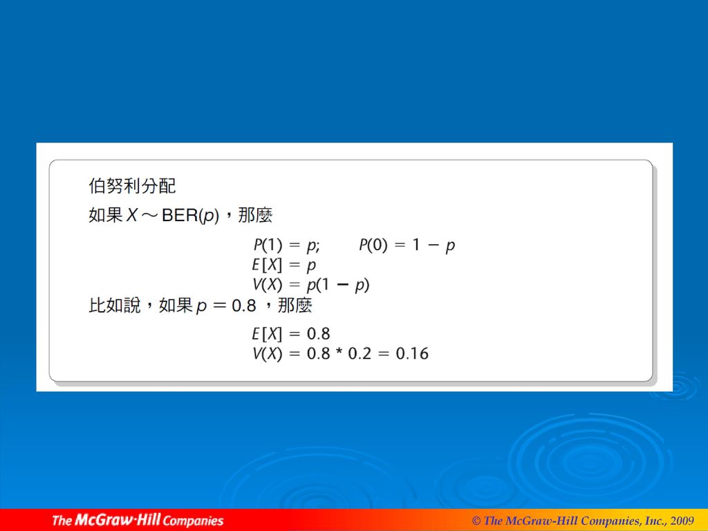
30 伯努利隨機變數 假設試驗的出象不是成功就是失敗，則該試驗就是一種伯努利試驗 (Bernoulli trial)。
一次伯努利試驗的成功次數（不是 1 就是 0）是一種伯努利隨機變數 (Bernoulli random variable)。 多次獨立同分配的伯努利試驗有幾次成功的變數，稱為二項隨機變數 (binomial random variable)。

31

32 二項隨機變數 定義：多次獨立同分配的伯努利試驗有幾次成功的變數 必須符合的條件： 每次伯努利試驗只有二種可能出象，不是「成功」就是「失敗」
試驗出象彼此獨立 每次試驗的成功機率固定保持不變

33 二項隨機變數

34 二項隨機變數

35 Mean, Variance, and Standard Deviation of the Binomial Distribution

36 Shape of the Binomial Distribution
y : n = 4 p = . 1 B i n o m i a l P r o b a b i l i t y : n = 4 p = . 3 B i n o m i a l P r o b a b i l i t y : n = 4 p = . 5 . 7 . 7 . 7 . 6 . 6 . 6 n = 4 . 5 . 5 . 5 ( ) x . 4 ( x ) . 4 ) . 4 P x ( . 3 P . 3 P . 3 . 2 . 2 . 2 . 1 . 1 . 1 . . . 1 2 3 4 1 2 3 4 1 2 3 4 x x x B i n o m i a l P r o b a b i l i t y : n = 1 p = . 1 B i n o m i a l P r o b a b i l i t y : n = 1 p = . 3 B i n o m i a l P r o b a b i l i t y : n = 1 p = . 5 . 5 . 5 . 5 . 4 . 4 . 4 n = 10 x ) . 3 ( ( ) x . 3 P P P x ( ) . 3 . 2 . 2 . 2 . 1 . 1 . 1 . . . 1 2 3 4 5 6 7 8 9 1 1 2 3 4 5 6 7 8 9 1 1 2 3 4 5 6 7 8 9 1 x x x B i n o m i a l P r o b a b i l i t y : n = 2 p = . 1 B i n o m i a l P r o b a b i l i t y : n = 2 p = . 3 B i n o m i a l P r o b a b i l i t y : n = 2 p = . 5 n = 20 2 . 2 . . 2 x ) ( x ( ) ) P P x P ( 1 . 1 . 1 . . . . 1 2 3 4 5 6 7 8 9 1 1 1 1 2 1 3 1 4 1 5 1 6 1 7 1 8 1 9 2 1 2 3 4 5 6 7 8 9 1 1 1 1 2 1 3 1 4 1 5 1 6 1 7 1 8 1 9 2 1 2 3 4 5 6 7 8 9 1 1 1 1 2 1 3 1 4 1 5 1 6 1 7 1 8 1 9 2 x x x Binomial distributions become more symmetric as n increases and as p

37 連續隨機變數 是一種可能等於某區間內任意數值的隨機變數 機率密度函數 f(x) 有下列性質 對所有 x， f(x) ≧0
X 落在 a 與 b 之間的機率等於 f(x) 下方在 a 與 b 之間的面積 整個函數 f(x) 下方的面積等於 1.00

38 舉例 某產品不良率為P=2%，今自一批貨中抽查100件，請問樣本中含有兩個及兩個以上不良品的機率為何？
某機器生產螺絲釘的不良率為20%，現在隨機抽取4個，令不良品為隨機變數X，試求其機率分配、期望值、變異數。

39 均勻分配 均勻分配是最簡單的連續分配。 機率密度函數定義為 f(x)=1/(b－a) a≦x≦b = 0 其他 x
其中 a 是 X 的最小可能值，b 是 X 的最大可能值。f(x)的圖如下頁。

40 均勻分配

41 均勻分配

42 均勻分配 某些會依某種循環時間重複出現的車輛，例如機場的接駁車或遊樂場的遊園車。
如果某位乘客隨意來到一處招呼站，等待車輛到來，則等待時間會是一個 0 與循環時間的均勻分配。 如果機場接駁車的循環時間是 20 分鐘，則等待時間會是 0 與 20 分鐘的均勻分配。