Time Frequency Analysis and Wavelet Transforms Oral Presentation

Presentation on theme: "Time Frequency Analysis and Wavelet Transforms Oral Presentation"— Presentation transcript:

1 Time Frequency Analysis and Wavelet Transforms Oral Presentation
Image Compression JPEG and JPEG 2000 Presenter：許銘宸 November 9,2017

2 Goal Save the memories Reduce the transmission time

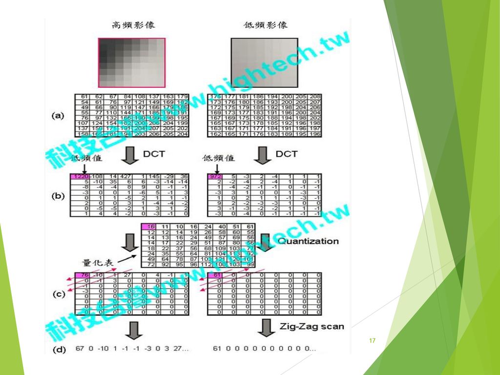
3 How Low frequency parts correlation between pixels→high sensitive for the human eyes ex：large area with the same color High frequency parts correlation between pixel→low insensitive for the human eyes ex：edge、corner High frequency parts are the information that we are uninterested

4 Evaluation Mean Square Error (MSE):
𝑀𝑆𝐸= 𝑥=0 𝑊−1 𝑦=0 𝐻−1 𝐼 𝑥,𝑦 −𝐾 𝑥,𝑦 𝑊𝐻 I(x,y): original image K(x,y): reconstructed imag H: height of image W: width of image Peak signal-to-noise ratio (PSNR): 𝑃𝑆𝑁𝑅=10 log 𝑀𝐴𝑋 𝐼 2 𝑀𝑆𝐸 𝑀𝐴𝑋 𝐼 :the maximum possible pixel value of the image

5 Flowchart of JPEG

6 Correlation between pixels

7 RGB to YCbCr Sensitivity for human eyes:
Red(R) > Green(G) > Blue(B) Luminance(Y) > Chrominance(Cb, Cr) 𝑌 =+0.299×𝑅+0.587×𝐺+0.114×𝐵 𝐶 𝑏 =−0.169×𝑅−0.331×𝐺+0.500×𝐵 𝐶 𝑟 =+0.500×𝑅−0.419×𝐺−0.081×𝐵

8 Downsampling Y Cb Cr Y Cb Cr Y Cb Cr or Y Cb Cr
4:4:4 (No downsampling) 4:2:2 (Downsampling every 2 pixels in vertical or horizontal direction.) 4:2:0(Downsampling every 2 pixels in both vertical and horizontal direction.) Y Cb Cr Y Cb Cr Y Cb Cr or Y Cb Cr

9 KL Transform & DCT Transform
Fourier Transform & Fourier Series (1-Dimension): combination of sines and cosines. KL Transform & DCT Transform (2-Dimension): combination of many kinds of simple pattern (i.e. bases).

10 KLT & DCT Karhunen-Loeve Transform (KLT): Every image has its own bases Advantage: Minimums the Mean Square Error(MSE). Disadvantage: We need to find the bases information → Computationally expensive. We need to save the bases information → More data. Discrete Cosine Transform (DCT): Compress different image by the “same” bases Computationally efficient. The performance of MSE is not as well as KL Transform But it’s good enough.

11 Formulas of DCT: DCT 𝐹 𝑢,𝑣 = 2𝐶 𝑢 𝐶 𝑣 𝑁 𝑖=0 𝑁−1 𝑗=0 𝑁−1 𝑓 𝑖,𝑗 cos 2𝑖+1 𝑢𝜋 2𝑁 cos 2𝑗+1 𝑣𝜋 2𝑁 Inverse-DCT 𝑓 𝑖,𝑗 = 2 𝑁 𝑢=0 𝑁−1 𝑣=0 𝑁−1 𝐶 𝑢 𝐶 𝑣 𝐹 𝑢,𝑣 cos 2𝑖+1 𝑢𝜋 2𝑁 cos 2𝑗+1 𝑣𝜋 2𝑁 Where 0≤𝑖,𝑗,𝑢,𝑣≤𝑁−1, 𝐶 𝑛 = 1 2 𝑛=0 1 𝑛≠0 For JPEG N=8

12 DCT bases

13 Example of DCT Before DCT: -76, -73, -67, -62, -58, -67, -64, -55,
-65, -69, -73, -38, -19, -43, -59, -56, -66, -69, -60, -15, 16, -24, -62, -55, -65, -70, -57, -6, 26, -22, -58, -59, -61, -67, -60, -24, -2, -40, -60, -58, -49, -63, -68, -58, -51, -60, -70, -53, -43, -57, -64, -69, -73, -67, -63, -45, -41, -49, -59, -60, -63, -52, -50, -34 After DCT: , , , , , , , , 4.47, , , , , , , , -46.83, , , , , , , , -48.53, , , , , , , , 12.13, , , , , , , , -7.73, , , , , , , , -1.03, , , , , , , , -0.17, , , , , , , ,

14 Quantization 𝐹 ′ 𝑢,𝑣 = 𝐹(𝑢,𝑣) 𝑄(𝑢,𝑣) +0.5 0≤𝑢,𝑣≤7
𝐹 ′ 𝑢,𝑣 = 𝐹(𝑢,𝑣) 𝑄(𝑢,𝑣) ≤𝑢,𝑣≤7 16 11 10 24 40 51 61 12 14 19 26 58 60 55 13 57 69 56 17 22 29 87 80 62 18 37 68 109 103 77 35 64 81 104 113 92 49 78 106 121 120 101 72 95 98 112 100 99 17 18 24 47 99 21 26 66 56 Luminance quantization table Chrominance quantization table

15 Example of Quantization
Before Quantization After Quantization , , , , , , , , 4.47, , , , , , , , -46.83, , , , , , , , -48.53, , , , , , , , 12.13, , , , , , , , -7.73, , , , , , , , -1.03, , , , , , , , -0.17, , , , , , , , Quantize by luminance quantization table -26, -3, -6, 2, 2, -1, 0, 0, 0, -2, -4, 1, 1, 0, 0, 0, -3, 1, 5, -1, -1, 0, 0, 0, -3, 1, 2, -1, 0, 0, 0, 0, 1, 0, 0, 0, 0, 0, 0, 0, 0, 0, 0, 0, 0, 0, 0, 0,

16 Zigzag Scan -26 -3 -6 2 -1 -2 -4 1 5 Zigzag Scan
-2 -4 1 5 Zigzag Scan We get a sequence after the zigzag process: −26, −3, 0, −3, −2, −6, 2, −4, 1 −3,-3, 1, 1, 5, 1, 2, −1, 1, −1, 2, 0, 0, 0, 0, 0, −1, −1, 0, ……,0. The sequence can be expressed as: (0:-26),(0:-3),(1:-3),…,(0:2),(5:-1),(0:-1),EOB Run-Length Encoding

17

18 Entropy Coding & Huffman Coding
Encode the high/low probability symbols with short/long code length. Symbol Binary Code 00 1 010 2 011 3 100 4 101 … 8 111110 9 10 11 Symbol Binary Code Run Size 1 00 … 10 6 15 EOB 1010 ZRL 1111 DC luminance Huffman Table AC luminance Huffman Table

19 Flowchart of JPEG2000

20 For high compression ratio
For JPEG 2000, there is no need to divide the image into many 8x8 blocks JPEG both has Strong block effect and blur JPEG-2000 only has blur

21 Forward Multicomponent Transformation
Irreversible component transform (ICT) ICT is used in the lossy compression , which is same as JPEG Reversible component transform (RCT) RCT is used in the lossy and lossless compression Y= R+2G+B 4 C b =B−G C r =R−G

22 Tiles Size：tile >> block
重點區塊處理（Region of Interest）：不同的區域可以挑選不同的壓縮品質

23 2D-DWT

24 A rectangular after 2D-DWT

25 The three stage 2D-DWT 遞進性（Progressive）： 解析度隨解碼長度遞增
可適性（Scaling）： 編碼內容可於任意位置截斷 當需要高壓縮率 →丟棄後方編碼資料

26 Inverse DWT

27 Cohen-Daubechies-Feauveau wavelet (CDF) filter
irreversible DWT is the CDF 9/7 wavelet filter reversible DWT is the CDF 5/3 wavelet filter

28 Quantization for JPEG 2000 , 𝑞 𝑏 𝑢,𝑣 =𝑠𝑖𝑔𝑛 𝑎 𝑏 𝑢,𝑣 ∗𝑓𝑙𝑜𝑜𝑟[ 𝑎 𝑏 (𝑢,𝑣) ∆ 𝑏 ] Step size： ∆ 𝑏 = 2 𝑅 𝑏 − 𝜀 𝑏 (1+ 𝜇 𝑏 ) R 𝑏 ：The nominal dynamic range of subband b 𝜀 𝑏 𝑎𝑛𝑑 𝜇 𝑏 ：Adjust the strength of quantization Lossless and lossy quantization can be achieved by different quantization step size For lossless quantization ： ∆ 𝑏 =1 when R 𝑏 =𝜀 𝑏 𝑎𝑛𝑑 𝜇 𝑏 =0

29 Tier-1 Encoder Embedded Block Coding
Code-block：32*32 or 64*64 Bit-plane：Bit depth → MSB(高位元) 到 LSB(低位元) Pass：每個位元層都再依「重要性」分為三個分流，分開套用內容統計模型 Pass1：最重要的資料，該處上一層還沒出現過最高有效位元但鄰近處出現者 Pass2：該位置已經出現過最高有效位元，對於較低位元繼續記錄其位元值 Pass3：該處上一層還沒出現過最高有效位元，且鄰近處也都不曾出現過

30 內容統計模型 (Context modeling)
零編碼（zero coding）： 用於分流一、三，紀錄非最高有效位元者。 正負號編碼（sign coding）： 用於分流一、三，紀錄出現最高有效位元者。 精細編碼（Magnitude refinement coding）： 用於分流二。 遊程編碼（Run-length coding）： 用於分流三，紀錄全都不是最高有效位元的狀況。

31 Tier-1 Encoder 算術編碼（Arithmetic coding）
Huffman coding 是將每一筆資料分開編碼 Arithmetic coding 則是將多筆資料一起編碼， 因此壓縮效率比 Huffman coding 更高，近年來的資料壓縮技術大 多使用 arithmetic coding

32 Arithmetic coding-range encoding

33 Arithmetic coding-range encoding
where C and b are integers (b is as small as possible), then the data X can be encoded by where means that using k-ary (k 進位) and b bits to express C. 0.4375 所以編碼的結果為

34 Rate control and Tier-2 encoder
Rate Control： Maintain the minimum distortion for the best image quality with the optimal bitrate to specify the image data size Tier-2 encoder： Packages the output of the Tier-1 encoder into the bit-stream.

35 Conclusion for JPEG We transfer RGB to YCbCr since the luminance is sensitive to the human eyes We reduce the correlation between pixels by applying DCT to concentrate the energy in DC term We quantize the DCT blocks to reduce the high frequency components (i.e.AC terms). We transfer the 8x8 blocks into sequence for purpose of run-length-coding We encode the sequences by Huffman-coding to minimize code length

36 Conclusion for JPEG-2000 We transfer RGB to YCbCr by ICT or RCT to choose lossy or lossless compression We perform DWT to split each tile into several subbands to reduce the correlation between pixels We quantize the DWT coefficients by adjusting the quantization step to achieve lossy or lossless compression We encode the quantized DWT coefficients by Tier-1 encoder, Tier-2 encoder and Rate Control with arithmetic coding to get a compressed image.

37 JPEG 2000 is not as popular as JPEG
For JPEG We have to input the entire image into the memory buffer of hardware. For JPEG It divides the image into several 8x8 blocks during the compression. The cost of memory for JPEG is small. JPEG 2000是基於小波變換的圖像壓縮標準。 JPEG 2000的壓縮比更高，而且不會產生原先的基於離散餘弦變換的JPEG標準產 生的塊狀模糊瑕疵。JPEG 2000同時支持破壞性資料壓縮和非破壞性資料壓縮。 另外，JPEG 2000也支持更複雜的漸進式顯示和下載。  由於JPEG 2000在非破壞性壓縮下仍然能有比較好的壓縮率，所以JPEG 2000在圖 像品質要求比較高的醫學圖像的分析和處理中已經有了一定程度的廣泛應用。

38 Reference [1] 酒井善則、吉田俊之 共著，白執善 編譯，影像壓縮技術 映像情報符号化， 全華科技圖書股份有限公司, Oct. 2004 [2] Discrete Wavelet Transform for JPEG 2000 [3] Tier 1 and Tier 2 Encoding Techniques for JPEG 2000 [4] WIKIPEDIA, “JPEG”, [5] WIKIPEDIA, “JPEG2000”,

39 The End