Download presentation
Presentation is loading. Please wait.

1
Ch.2 Modeling in the Frequency Domain

2
學習成果 Learning Outcomes
學習Transfer function技術:含Laplace transform、由「微分方程」求「transfer function」、由「transfer function」解 「微分方程」( ) 求線性、非時變電路系統的「轉移函數」 (2.4) 求線性、非時變移動機械系統的「轉移函數」 (2.5) 求線性、非時變轉動機械系統的「轉移函數」 (2.6) 求齒輪系統的「轉移函數」 (2.7) 求線性、非時變機電系統的「轉移函數」 (2.8) 機械系統的電路模擬(2.9) 非線性系統的線性化技術,為求「轉移函數」 ( )
 求線性、非時變電路系統的「轉移函數」 (2.4) 求線性、非時變移動機械系統的「轉移函數」 (2.5) 求線性、非時變轉動機械系統的「轉移函數」 (2.6) 求齒輪系統的「轉移函數」 (2.7) 求線性、非時變機電系統的「轉移函數」 (2.8) 機械系統的電路模擬(2.9) 非線性系統的線性化技術,為求「轉移函數」 ( )")
3
求「轉移函數」的目的:

4
天線模型 → 天線運動的微分方程式 → 天線的位移方程式
天線模型 → 天線運動的微分方程式 → 天線的位移方程式

5
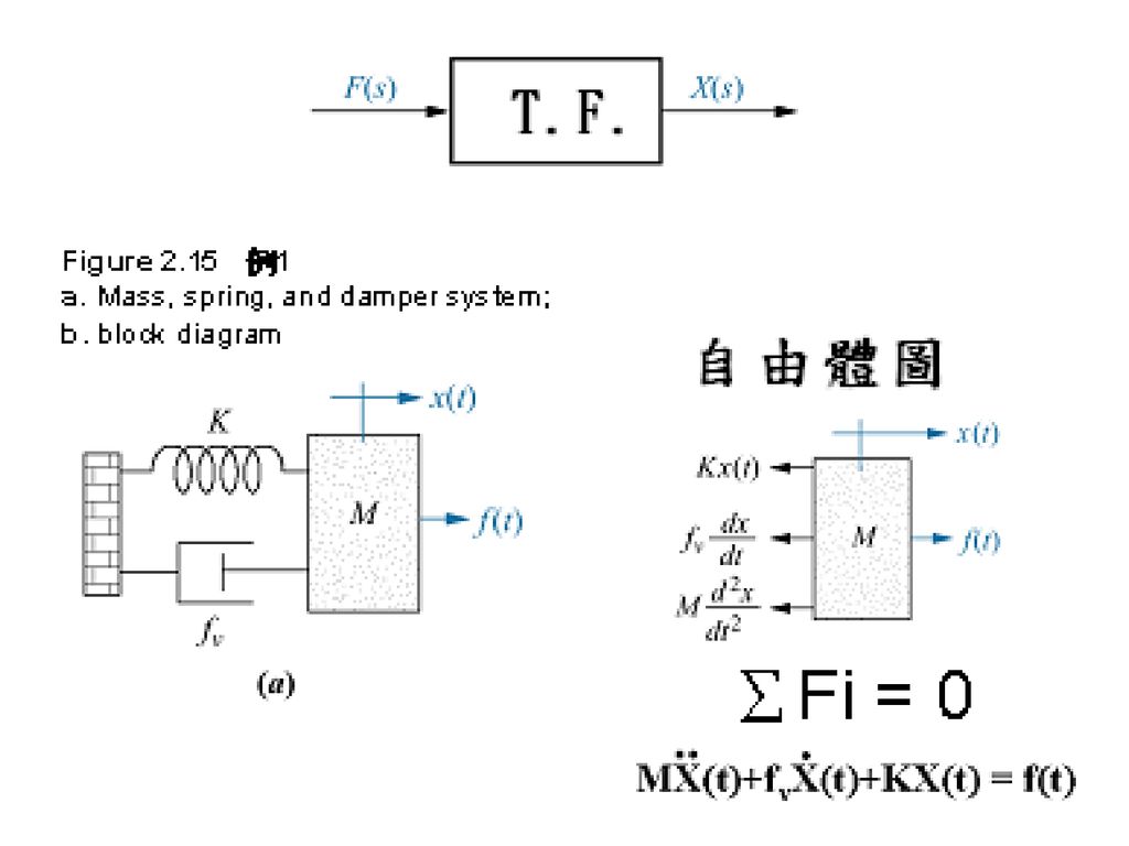
以牛頓第二定律為例: F(t) = M a(t)
Taking Laplace: F(t) = M a(t) → F(s) = M a(s) 所有初始條件= 0 Output/input = 1/M; a/F = 1/M ; F(s) = M a(s)
 = M a(t) → F(s) = M a(s) 所有初始條件= 0. Output/input = 1/M; a/F = 1/M ; F(s) = M a(s)")
6
Output = Transfer function × Input

9
Taking inverse Laplace: X(s) → X(t)
 → X(t)")
13
Table 1.1 (測試系統性能的輸入指令) Test waveforms used in control systems
 Test waveforms used in control systems")
14
物理意義 拍一下 定力拉 變力拉 (固定增幅) 變力拉 (加速增幅) Sin 變力
 變力拉 (加速增幅) Sin 變力")
15
Table 2.1 Laplace transform table

16
Table 2.2 Laplace transform theorems

17
學習成果 Learning Outcomes
學習Transfer function技術:含Laplace transform、由「微分方程」求「transfer function」、由「transfer function」解 「微分方程」( ) 求線性、非時變電路的「轉移函數」 (2.4) 求線性、非時變移動機械系統的「轉移函數」 (2.5) 求線性、非時變轉動機械系統的「轉移函數」 (2.6) 求齒輪系統的「轉移函數」 (2.7) 求線性、非時變機電系統的「轉移函數」 (2.8) 機械系統的電路模擬(2.9) 非線性系統的線性化技術,為求「轉移函數」 ( )
 求線性、非時變電路的「轉移函數」 (2.4) 求線性、非時變移動機械系統的「轉移函數」 (2.5) 求線性、非時變轉動機械系統的「轉移函數」 (2.6) 求齒輪系統的「轉移函數」 (2.7) 求線性、非時變機電系統的「轉移函數」 (2.8) 機械系統的電路模擬(2.9) 非線性系統的線性化技術,為求「轉移函數」 ( )")
18
§ 2.5 Translational Mechanical System
Transfer Functions 阻抗的觀念(in S)
")
19
阻抗觀念

20
阻尼器 Damper

21
一維系統

22
阻抗觀念 求系統方程式

24
Figure 2.17 a. Two-degrees-of-freedom translational mechanical system; b. block diagram
需2方程式描述系統之運動 A X1(s) + B X2(s) = F(s) C X1(s) + D X2(s) = 0 二維系統
 + B X2(s) = F(s) C X1(s) + D X2(s) = 0. 二維系統.")
25
A X1(s) + B X2(s) = F(s) Equation of Motion of M1 Σ外力=0 牛頓第二定律
Figure 2.18 Equation of Motion of M1 M1’s Free Body Diagram a. Forces on M1 due only to motion of M1; 即 M1移X1、 M2固定時,M1之受力 b. forces on M1 due only to motion of M2; 即 M2移X2、M1固定時,M1之受力 c. all forces on M1 M1受力之自由體圖 Σ外力=0 牛頓第二定律 A X1(s) + B X2(s) = F(s) Eq a P.66
 + B X2(s) = F(s) Eq a P.66.")
26
C X1(s) + D X2(s) = 0 Figure 2.19 Equation of Motion of M2
M2’s Free Body Diagram a. Forces on M2 due only to motion of M2; 即 M2移X2、 M1固定時,M2之受力 b. forces on M2 due only to motion of M1; 即 M1移X1、 M2固定時,M2之受力 c. all forces on M2 M2受力之自由體圖 Σ外力=0 牛頓第二定律 C X1(s) + D X2(s) = 0 Eq b P.66
 + D X2(s) = 0. Eq b P.66.")
27
System equation P.66 A X1(s) + B X2(s) = F(s) a C X1(s) + D X2(s) = b 解2元1次聯立方程式 (By Cremer’s Rule) X2(s)/ F(s) = G(s) (2.119)
 X2(s)/ F(s) = G(s) (2.119)")
28
P.67 由公式(2.120a; 2.120b) 直接求系統方程式 A X1(s) + B X2(s) = F(s) 2.118a
C X1(s) + D X2(s) = b
 + D X2(s) = b.")
29
Figure 2.21 Translational mechanical system for Skill-Assessment Exercise 2.8
P.67 由牛頓第二定律求系統方程式

30
Figure 2.20 Three-degrees-of-freedom translational mechanical system

31
P.68 由公式( ) 直接求系統方程式
 直接求系統方程式")
33
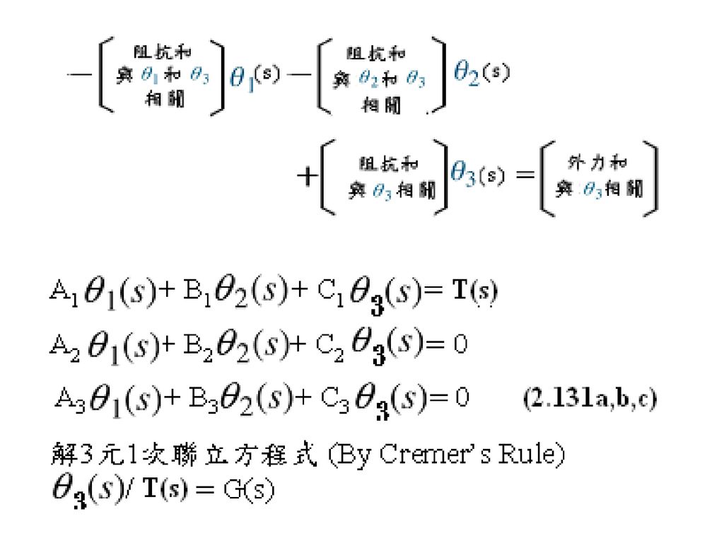
A1 X1(s) + B1 X2(s) + C1 X3(s) = 0 (2.124)
A2 X1(s) + B2X2(s) + C2 X3(s) = F(s) (2.125) A3 X1(s) + B3X2(s) + C3 X3(s) = (2.126) 解3元1次聯立方程式 (By Cremer’s Rule) X3(s)/ F(s) = G(s)
 + B2X2(s) + C2 X3(s) = F(s) (2.125) A3 X1(s) + B3X2(s) + C3 X3(s) = 0 (2.126) 解3元1次聯立方程式 (By Cremer’s Rule) X3(s)/ F(s) = G(s)")
34
A1 X1(s) + B1 X2(s) + C1 X3(s) = 0 (2.124)
A2 X1(s) + B2X2(s) + C2 X3(s) = F(s) (2.125) A3 X1(s) + B3X2(s) + C3 X3(s) = (2.126) 解3元1次聯立方程式 (By Cremer’s Rule) X3(s)/ F(s) = G(s)
 + B2X2(s) + C2 X3(s) = F(s) (2.125) A3 X1(s) + B3X2(s) + C3 X3(s) = 0 (2.126) 解3元1次聯立方程式 (By Cremer’s Rule) X3(s)/ F(s) = G(s)")
35
§2.6 Rotational Mechanical System Week 3

36
學習成果 Learning Outcomes
學習Transfer function技術:含Laplace transform、由「微分方程」求「transfer function」、由「transfer function」解 「微分方程」( ) 求線性、非時變電路的「轉移函數」 (2.4) 求線性、非時變移動機械系統的「轉移函數」 (2.5) 求線性、非時變轉動機械系統的「轉移函數」 (2.6) 求齒輪系統的「轉移函數」 (2.7) 求線性、非時變機電系統的「轉移函數」 (2.8) 機械系統的電路模擬(2.9) 非線性系統的線性化技術,為求「轉移函數」 ( )
 求線性、非時變電路的「轉移函數」 (2.4) 求線性、非時變移動機械系統的「轉移函數」 (2.5) 求線性、非時變轉動機械系統的「轉移函數」 (2.6) 求齒輪系統的「轉移函數」 (2.7) 求線性、非時變機電系統的「轉移函數」 (2.8) 機械系統的電路模擬(2.9) 非線性系統的線性化技術,為求「轉移函數」 ( )")
38
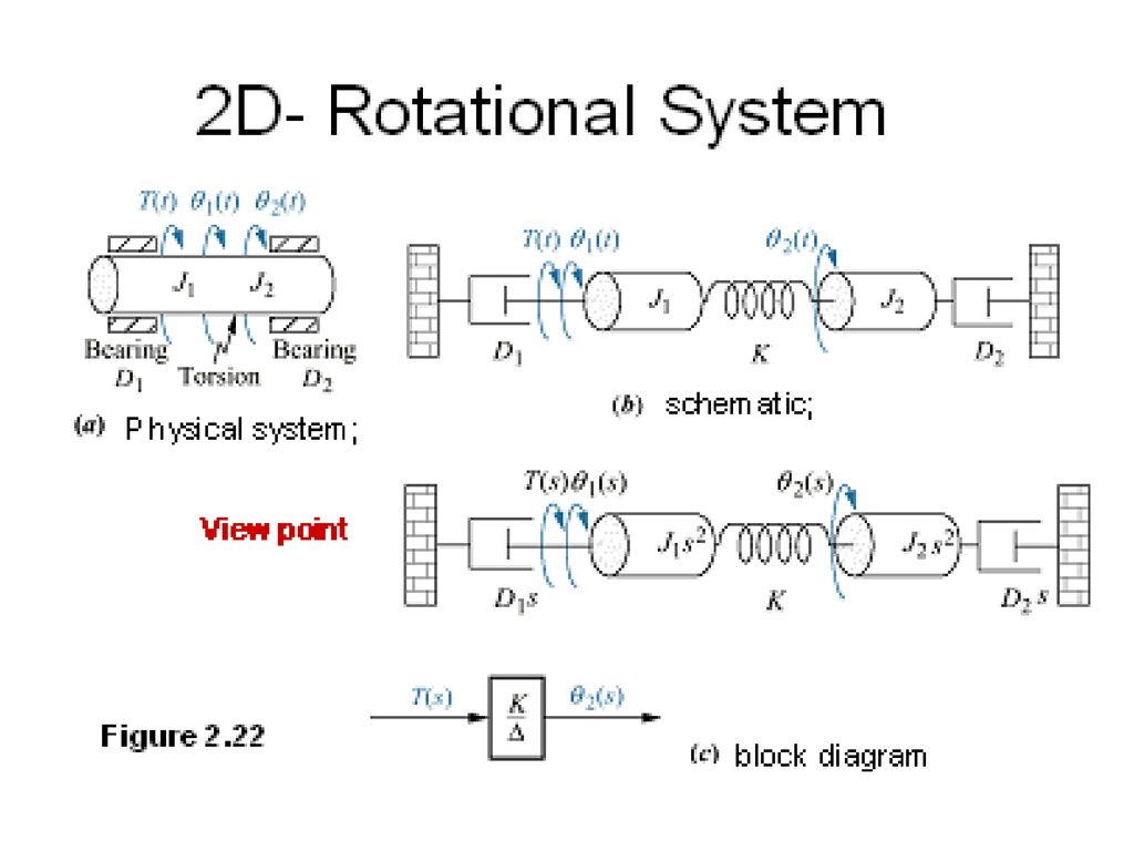
1D- Rotational System

39
1D- Rotational System

40
轉動慣量 J 的求法? 查 「應用力學」

42
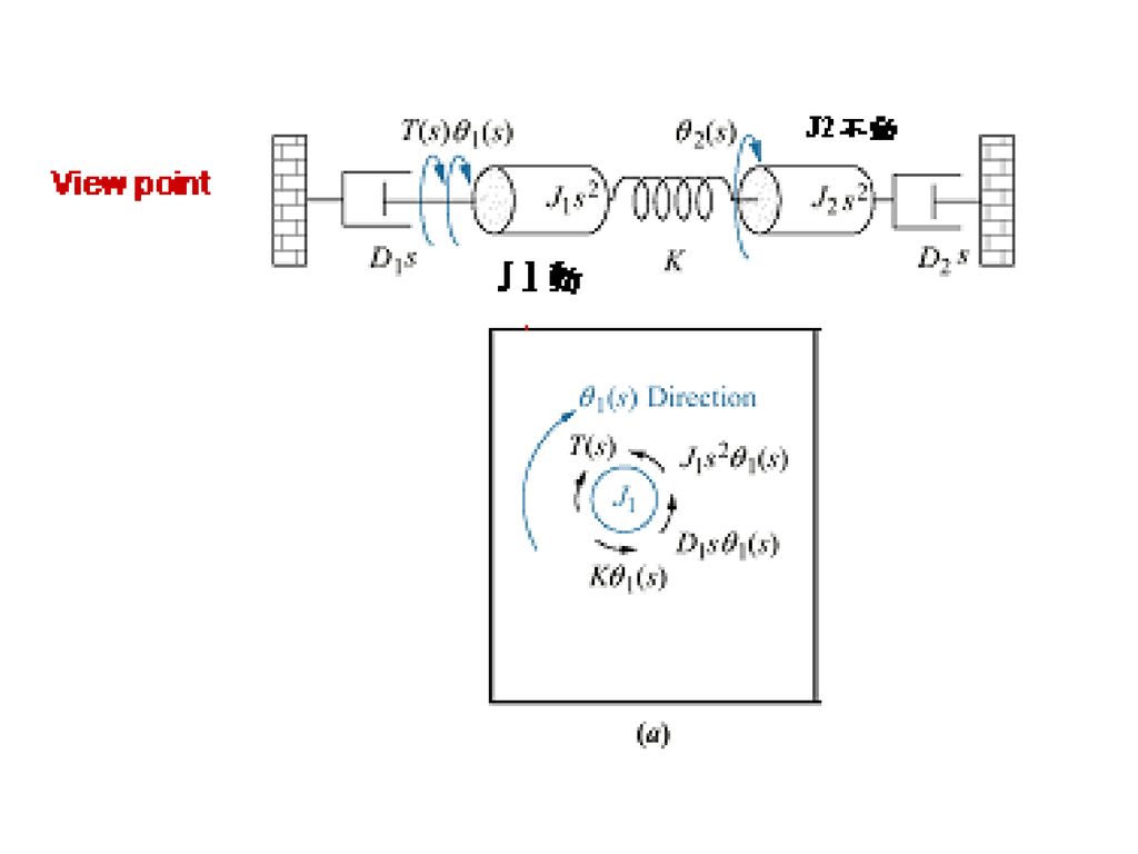
(J1S2 + D1S + K) θ1(s) - K θ2(s) = T(s) (2.127a)
View point Equation of motion for J1 (J1S2 + D1S + K) θ1(s) - K θ2(s) = T(s) (2.127a) Figure a. Torques on J1 due only to the motion of J1 J1動 J2不動 b. torques on J1 due only to the- motion of J J1不動 J2動 c. final free-body diagram for J1
 θ1(s) - K θ2(s) = T(s) (2.127a) Figure 2.23 a. Torques on J1 due only to the motion of J1 J1動 J2不動 b. torques on J1 due only to the- motion of J2 J1不動 J2動 c. final free-body diagram for J1.")
45
(J1S2 + D1S + K) θ1(s) - K θ2(s) = T(s) (2.127a)
View point Equation of motion for J1 (J1S2 + D1S + K) θ1(s) - K θ2(s) = T(s) (2.127a) Figure a. Torques on J1 due only to the motion of J1 J1動 J2不動 b. torques on J1 due only to the- motion of J J1不動 J2動 c. final free-body diagram for J1
 θ1(s) - K θ2(s) = T(s) (2.127a) Figure 2.23 a. Torques on J1 due only to the motion of J1 J1動 J2不動 b. torques on J1 due only to the- motion of J2 J1不動 J2動 c. final free-body diagram for J1.")
46
外力和=o: - K θ1(s) + (J2S2 + D2S + K) θ2(s) = 0 (2.127b)
View point Equation of motion for J2 外力和=o: - K θ1(s) + (J2S2 + D2S + K) θ2(s) = (2.127b) Figure a. Torques on J2 due only to the motion of J J1不動 J2動 b. torques on J2 due only to the motion of J J1動 J2不動 c. final free-body diagram for J2
 + (J2S2 + D2S + K) θ2(s) = 0 (2.127b) Figure 2.24 a. Torques on J2 due only to the motion of J2 J1不動 J2動 b. torques on J2 due only to the motion of J1 J1動 J2不動 c. final free-body diagram for J2.")
47
Find T.F. (J1S2 + D1S + K) θ1(s) - K θ2(s) = T(s) (2.127a) - K θ1(s) + (J2S2 + D2S + K) θ2(s) = (2.127b) By Cremer’s Rule → θ2(s) = (K/△) T(s) T.F. G(s) = (eq )
 θ1(s) - K θ2(s) = T(s) (2.127a) - K θ1(s) + (J2S2 + D2S + K) θ2(s) = 0 (2.127b) By Cremer’s Rule → θ2(s) = (K/△) T(s) T.F. G(s) = (eq )")
48
Ex. 2.20 3-D rotational system
Figure 2.25 Three-degrees-of-freedom rotational system Equation of Motion: 公式 2.130a,b,c 直接寫出 如2.131a,b,c

51
Find T.F. G(s) = θ2(s) / T(s)
Figure Homework Rotational mechanical system for Skill-Assessment Exercise 2.9

52
Week 4

53
學習成果 Learning Outcomes
學習Transfer function技術:含Laplace transform、由「微分方程」求「transfer function」、由「transfer function」解 「微分方程」( ) 求線性、非時變電路的「轉移函數」 (2.4) 求線性、非時變移動機械系統的「轉移函數」 (2.5) 求線性、非時變轉動機械系統的「轉移函數」 (2.6) 求齒輪系統的「轉移函數」 (2.7) 求線性、非時變機電系統的「轉移函數」 (2.8) 機械系統的電路模擬(2.9) 非線性系統的線性化技術,為求「轉移函數」 ( )
 求線性、非時變電路的「轉移函數」 (2.4) 求線性、非時變移動機械系統的「轉移函數」 (2.5) 求線性、非時變轉動機械系統的「轉移函數」 (2.6) 求齒輪系統的「轉移函數」 (2.7) 求線性、非時變機電系統的「轉移函數」 (2.8) 機械系統的電路模擬(2.9) 非線性系統的線性化技術,為求「轉移函數」 ( )")
55
By Kirchhoff’s Voltage Law
Figure 2.3 1D Network RLC network By Kirchhoff’s Voltage Law △VL+△VR + △VC + V(t) = 0
 = 0.")
56
Figure 2.3 RLC network

57
Figure 2.3 RLC network G(s)
")
58
2D Network Find T.F. : Vc / V Figure 2.6 Two-loop electrical network
Kirchhoff’s Voltage Law Input: V Responses: i1, i2 Find T.F. : Vc / V 需2方程式描述系統之狀態 方程式1: Loop i1 方程式2 : Loop i2

59
2D Network

60
2D Network Kirchhoff’s Voltage Law 方程式1: Loop I1 R1 I1 – Ls(I1-I2) + V(s) = 0 → (R1+Ls) I1 – Ls I2 = V(s) 方程式2 : Loop I2 R2 I2 – I2/Cs - Ls(I2-I1) = 0 → – Ls I1 +【Ls + R2 + (1/Cs)】I2 = 0
 = 0 → – Ls I1 +【Ls + R2 + (1/Cs)】I2 = 0.")
61
2D Network (R1+Ls) I – Ls I2 = V(s) – Ls I 【Ls + R2 + (1/Cs)】I2 = 0
 I1 – Ls I2 = V(s) – Ls I1 +【Ls + R2 + (1/Cs)】I2 = 0.")
62
Figure 2.7 Block diagram of the network of Figure 2.6 T.F. : Vc / V
Vc(s) = (1/Cs) I2
 = (1/Cs) I2.")
63
Figure 2.9 Three-loop electrical network
3D Network

65
範例:外力在Mesh 2 A1I1(s) + B1I2(s) + C1I3(s) = (2.91) A2I1(s) + B2I2(s) + C2I3(s) = F(s) (2.92) A3I1(s) + B3I2(s) + C3I3(s) = (2.93) 解3元1次聯立方程式 (By Cremer’s Rule) I3(s)/ F(s) = G(s)
 + B3I2(s) + C3I3(s) = 0 (2.93) 解3元1次聯立方程式 (By Cremer’s Rule) I3(s)/ F(s) = G(s)")
66
Figure 2. 14 Electric circuit for kill-Assessment Exercise 2
Figure Electric circuit for kill-Assessment Exercise 2.6 Find G(s) = VL(s) / V(s) Homework
 = VL(s) / V(s) Homework.")
70
Figure 2.11 Homework Inverting operational amplifier circuit for Example 2.14

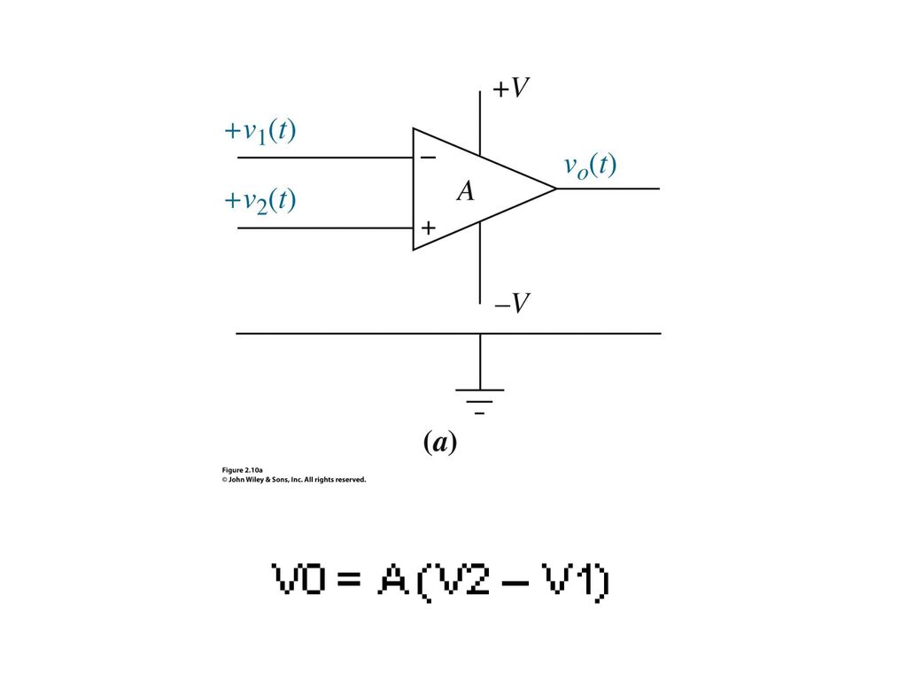
71
V0 = A (Vi – V1) V1 = 【 V0/(Z1 + Z2) 】Z1 ∵ A ﹥﹥1 V0/Vi = (Z1+Z2)/Z1
Figure General noninverting operational amplifier circuit V0 = A (Vi – V1) V1 = 【 V0/(Z1 + Z2) 】Z1 ∵ A ﹥﹥1 V0/Vi = (Z1+Z2)/Z1
 V1 = 【 V0/(Z1 + Z2) 】Z1 ∵ A ﹥﹥1 V0/Vi = (Z1+Z2)/Z1.")
72
Find G(s) = V0/Vi Figure Homework Noninverting operational amplifier circuit for Example 2.15
 = V0/Vi Figure 2.13 Homework Noninverting operational amplifier circuit for Example")
73
Quiz on Oct. 8th 2010 Find G(s) = VL(s) / V(s)
 = VL(s) / V(s)")
74
學習成果 Learning Outcomes
學習Transfer function技術:含Laplace transform、由「微分方程」求「transfer function」、由「transfer function」解 「微分方程」( ) 求線性、非時變電路的「轉移函數」 (2.4) 求線性、非時變移動機械系統的「轉移函數」 (2.5) 求線性、非時變轉動機械系統的「轉移函數」 (2.6) 求齒輪系統的「轉移函數」 (2.7) 求線性、非時變機電系統的「轉移函數」 (2.8) 機械系統的電路模擬(2.9) 非線性系統的線性化技術,為求「轉移函數」 ( )
 求線性、非時變電路的「轉移函數」 (2.4) 求線性、非時變移動機械系統的「轉移函數」 (2.5) 求線性、非時變轉動機械系統的「轉移函數」 (2.6) 求齒輪系統的「轉移函數」 (2.7) 求線性、非時變機電系統的「轉移函數」 (2.8) 機械系統的電路模擬(2.9) 非線性系統的線性化技術,為求「轉移函數」 ( )")
75
§ T.F. for Gear System 1/4 Figure A gear system

76
§ 2.7 T.F. for Gear System 2/4 r1θ1 = r2θ2 → N1θ1 = N2θ2
Figure Transfer functions for a. angular displacement in lossless gears

77
§ 2.7 T.F. for Gear System 3/4 → T1N2 = T2N1 T1θ1 = T2θ2
Figure Transfer functions for b. torque in lossless gears

78
T. F. for angular displacement
§ T.F. for Gear System 4/4 Figure A gear system Figure 2.28 T. F. for angular displacement in lossless gears T. F. for torque in lossless gears

79
註1: T.F. for Gear System Θ1 > θ ? Θ1 < θ ?

80
註2: T.F. for Gear System T1 > T ? T1 < T ?

81
省略齒輪組後的等效阻抗推導 (a) → (c) 1/5
Figure 2.29 a. Rotational system driven by gears; b. equivalent system at the output after reflection of input torque; c. equivalent system at the input after reflection of impedances

82
2/5 + → Case I

83
→ + → 3/5 T.F. G(s) = θ2(s) / T1(s) (JS2 + DS + K) θ2(s) = T1(s)
Case II

84
4/5 省略齒輪組的等效阻抗 (結論) 等效系統 →
 等效系統 →")
85
5/5

86
Figure 2.31 T.F. of Gear train

87
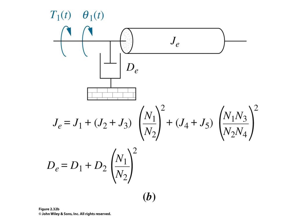
Figure 2. 32 Example 2. 22 HOMEWORK 證明 Je and De; 求 G(s)=θ1/T1 a
Figure Example HOMEWORK 證明 Je and De; 求 G(s)=θ1/T1 a. System using a gear train; b. equivalent system at the input; c. block diagram
=θ1/T1 a. System using a gear train; b. equivalent system at the input; c. block diagram.")
88
原系統 等效系統 Je = J1∪ J2 ∪ J3 ∪ J4 ∪ J5 對系統的綜合影響相同 De = D1∪ D 對系統的綜合影響相同 綜合影響相同 = 施相同外力T1 獲相同反應θ1

89
原系統 等效系統

90
在θ1軸感到的慣量 在θ1軸感到的阻尼

91
等效系統

93
Figure 2. 32 Example 2. 22 HOMEWORK 證明 Je and De; 求 G(s)=θ1/T1 a
Figure Example HOMEWORK 證明 Je and De; 求 G(s)=θ1/T1 a. System using a gear train; b. equivalent system at the input; c. block diagram
=θ1/T1 a. System using a gear train; b. equivalent system at the input; c. block diagram.")
94
Figure HOMEWORK Rotational mechanical system with gears for Skill-assessment Exercise 求 G(s)=θ2/T
=θ2/T")
95
→ 齒輪可省力 (證明) 等效系統 於等效系統中 J, D, K 均降為原負載的 1/ 4 If N1 / N2 = 1/ 2
齒輪可省力 (證明) 等效系統 → 於等效系統中 J, D, K 均降為原負載的 1/ 4 If N1 / N2 = 1/ 2 小齒輪驅動大齒輪
 等效系統. → 於等效系統中. J, D, K 均降為原負載的 1/ 4. If N1 / N2 = 1/ 2. 小齒輪驅動大齒輪.")
96
學習成果 Learning Outcomes
學習Transfer function技術:含Laplace transform、由「微分方程」求「transfer function」、由「transfer function」解 「微分方程」( ) 求線性、非時變電路的「轉移函數」 (2.4) 求線性、非時變移動機械系統的「轉移函數」 (2.5) 求線性、非時變轉動機械系統的「轉移函數」 (2.6) 求齒輪系統的「轉移函數」 (2.7) 求線性、非時變機電系統的「轉移函數」 (2.8) 機械系統的電路模擬(2.9) 非線性系統的線性化技術,為求「轉移函數」 ( )
 求線性、非時變電路的「轉移函數」 (2.4) 求線性、非時變移動機械系統的「轉移函數」 (2.5) 求線性、非時變轉動機械系統的「轉移函數」 (2.6) 求齒輪系統的「轉移函數」 (2.7) 求線性、非時變機電系統的「轉移函數」 (2.8) 機械系統的電路模擬(2.9) 非線性系統的線性化技術,為求「轉移函數」 ( )")
97
§2.8 T.F. of Electromechanical System
Figure NASA flight simulator robot arm with electromechanical control system components (an example)
")
98
Typical Example 1/10 Figure DC motor: a. schematic12; b. block diagram (T.F.) Figure 2.36 Typical equivalent mechanical loading on a motor Figure System DC motor driving a rotational mechanical load

99
求機電系統的T.F. G(s) /10 νb (t) = κb (dθm/dt) νb(t) : back emf 反電動勢 ; Κb : back emf constant dθm/dt : angular velocity of motor
 = κb (dθm/dt) νb(t) : back emf 反電動勢 ; Κb : back emf constant dθm/dt : angular velocity of motor.")
100
求機電系統的T.F. G(s) /10 Tm(t) = κt ia(t) Tm(t) : torque developed by motor ; Κt : motor torque constant ; ia(t) : armature current
 = κt ia(t) Tm(t) : torque developed by motor ; Κt : motor torque constant ; ia(t) : armature current.")
101
求機電系統的T.F. G(s) /10 νb(t) = κb (dθm/dt) νb(t) : back emf 反電動勢 ; Κb : back emf constant dθm/dt : angular velocity of motor Tm(t) = κt ia(t) Tm(t) : torque developed by motor ; Κt : motor torque constant ; ia(t) : armature current
 = κb (dθm/dt) νb(t) : back emf 反電動勢 ; Κb : back emf constant dθm/dt : angular velocity of motor Tm(t) = κt ia(t) Tm(t) : torque developed by motor ; Κt : motor torque constant ; ia(t) : armature current.")
102
5/10 ↓ Laplace

103
求機電系統的T.F. G(s) /10 By Kirchhoff’s current law -RaIa(s) – LasIa(s) – Vb(s) + Ea(s) = 0 外加電壓與Tm ,θm 關係 (Ra+Las) Tm(s) / Κt + Κbsθm(s) = Ea(s) (2.149)
 – LasIa(s) – Vb(s) + Ea(s) = 0 外加電壓與Tm ,θm 關係 (Ra+Las) Tm(s) / Κt + Κbsθm(s) = Ea(s) (2.149)")
104
求機電系統的T.F. G(s) 6/10 Motor 轉子 機械系統
機電系統 機械負載部 外力 : Tm ,θm (機與電共有的項目) θm 受機械負載影響 目標 找Ea 與θm 關係
 θm 受機械負載影響 目標 找Ea 與θm 關係.")
105
↓Laplace Jm = Ja + JL(N1/N2)2 Dm = Da + DL(N1/N2)2 外力 = Σ阻抗 * 反應
7/10 Jm = Ja + JL(N1/N2)2 Dm = Da + DL(N1/N2)2 ↓Laplace 外力 = Σ阻抗 * 反應 (JmS2 + DmS)θm(s) = Tm(s) By Newton’s 2nd Law JmS2θm(s) + DmSθm(s) = Tm(s) (2.150)
2 Dm = Da + DL(N1/N2)2. ↓Laplace. 外力 = Σ阻抗 * 反應. (JmS2 + DmS)θm(s) = Tm(s) By Newton’s 2nd Law JmS2θm(s) + DmSθm(s) = Tm(s) (2.150)")
106
8/10 JmS2θm(s) + DmSθm(s) = Tm(s) (2.150) By Newton’s 2nd Law (Ra+LaS) Tm(s) / Κt + ΚbSθm(s) = Ea(s) (2.149) (2.150) 代入 (2.149) (Ra+LaS) (JmS2 + DmS)θm(s) / Κt + ΚbSθm(s) = Ea(s) (2.151) Sice Ra>>La (Ra+LaS) → Ra usually true i.e. La= 0 (Ra/ Κt ) (JmS2 + DmS)θm(s) + ΚbSθm(s) = Ea(s) (2.152)
 + DmSθm(s) = Tm(s) (2.150) By Newton’s 2nd Law (Ra+LaS) Tm(s) / Κt + ΚbSθm(s) = Ea(s) (2.149) (2.150) 代入 (2.149) (Ra+LaS) (JmS2 + DmS)θm(s) / Κt + ΚbSθm(s) = Ea(s) (2.151) Sice Ra>>La (Ra+LaS) → Ra usually true i.e. La= 0 (Ra/ Κt ) (JmS2 + DmS)θm(s) + ΚbSθm(s) = Ea(s) (2.152)")
107
9/10 (Ra / Κt ) (JmS2 + DmS)θm(s) + ΚbSθm(s) = Ea(s) (2.152) G(s) = θm(s) / Ea(s) = κ / S(S+α) (2.154) κ= Κt / (Ra Jm) α= (Dm + Κt Κb / Ra) / Jm if κ,α已知 G(s) 完全定義 κ,α為已知 if Κt, Kb已知 求Κt , Kb?
 (JmS2 + DmS)θm(s) + ΚbSθm(s) = Ea(s) (2.152) G(s) = θm(s) / Ea(s) = κ / S(S+α) (2.154) κ= Κt / (Ra Jm) α= (Dm + Κt Κb / Ra) / Jm if κ,α已知 G(s) 完全定義 κ,α為已知 if Κt, Kb已知 求Κt , Kb")
108
求Κt , Kb. (Ra+LaS) Tm(s) / Κt + ΚbSθm(s) = Ea(s) (2
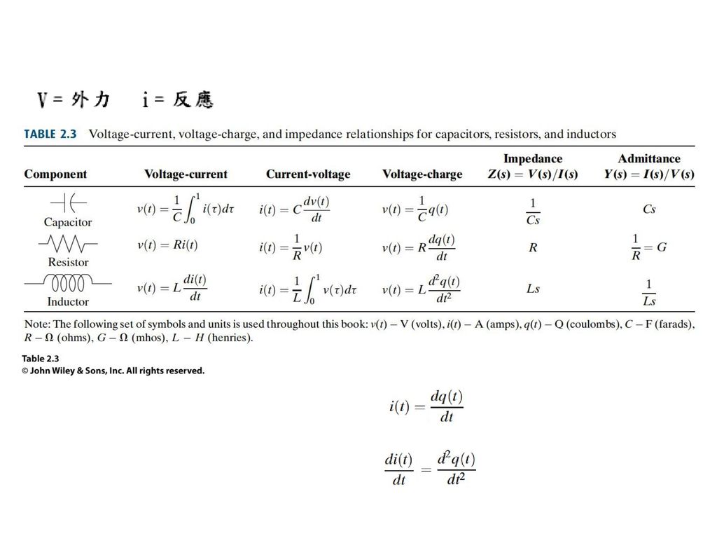
求Κt , Kb? (Ra+LaS) Tm(s) / Κt + ΚbSθm(s) = Ea(s) (2.149) RaTm(s) / Κt + ΚbSθm(s) = Ea(s) (La= 0) RaTm(t) / Κt + Κbωm(t) = ea(t) (after inverse Laplace) RaTm / Κt + Κbωm = ea (at steady state; ea :DC voltage) (aTm + bωm = 常數) (ax + by = 常數) 10/10 Figure 2.38 Torque-speed curves with an armature voltage, ea, as a parameter At Tstall where ωm= 0 → Κt At ωno-load where Tm = 0 → Κb Dynamometer: 於定電壓下量torque and speed of a motor
 Tm(s) / Κt + ΚbSθm(s) = Ea(s) (2.149) RaTm(s) / Κt + ΚbSθm(s) = Ea(s) (La= 0) RaTm(t) / Κt + Κbωm(t) = ea(t) (after inverse Laplace) RaTm / Κt + Κbωm = ea (at steady state; ea :DC voltage) (aTm + bωm = 常數) (ax + by = 常數) 10/10. Figure 2.38 Torque-speed curves with an armature voltage, ea, as a parameter. At Tstall where ωm= 0 → Κt At ωno-load where Tm = 0 → Κb Dynamometer: 於定電壓下量torque and speed of a motor.")
109
求Κt , Kb? RaTm / Κt + Κbωm = ea (at steady state; ea :DC voltage) (aTm + bωm = 常數) (ax + by = 常數)
10/10 At Tstall where ωm= 0 → Κt At ωno-load where Tm = 0 → Κb Dynamometer: 於定電壓下量torque and speed of a motor Figure 2.38 Torque-speed curves with an armature voltage, ea, as a parameter

110
Example 2.23 Homework 求Κt , Kb
Figure 2.39 a. DC motor and load; b. torque-speed curve; c. block diagram

111
Figure Homework Electromechanical system for Skill-Assessment Exercise 2.11 Find G(s) = θL(s)/Ea(s) Tm = -8ωm + 200

112
學習成果 Learning Outcomes
學習Transfer function技術:含Laplace transform、由「微分方程」求「transfer function」、由「transfer function」解 「微分方程」( ) 求線性、非時變電路的「轉移函數」 (2.4) 求線性、非時變移動機械系統的「轉移函數」 (2.5) 求線性、非時變轉動機械系統的「轉移函數」 (2.6) 求齒輪系統的「轉移函數」 (2.7) 求線性、非時變機電系統的「轉移函數」 (2.8) 機械系統的電路模擬(2.9) 非線性系統的線性化技術,為求「轉移函數」 ( )
 求線性、非時變電路的「轉移函數」 (2.4) 求線性、非時變移動機械系統的「轉移函數」 (2.5) 求線性、非時變轉動機械系統的「轉移函數」 (2.6) 求齒輪系統的「轉移函數」 (2.7) 求線性、非時變機電系統的「轉移函數」 (2.8) 機械系統的電路模擬(2.9) 非線性系統的線性化技術,為求「轉移函數」 ( )")
113
§2.9 Electric Circuit Analogs 1/3

114
§2.9 Electric Circuit Analogs 2/3
Laplace →

115
§2.9 Electric Circuit Analogs 3/3
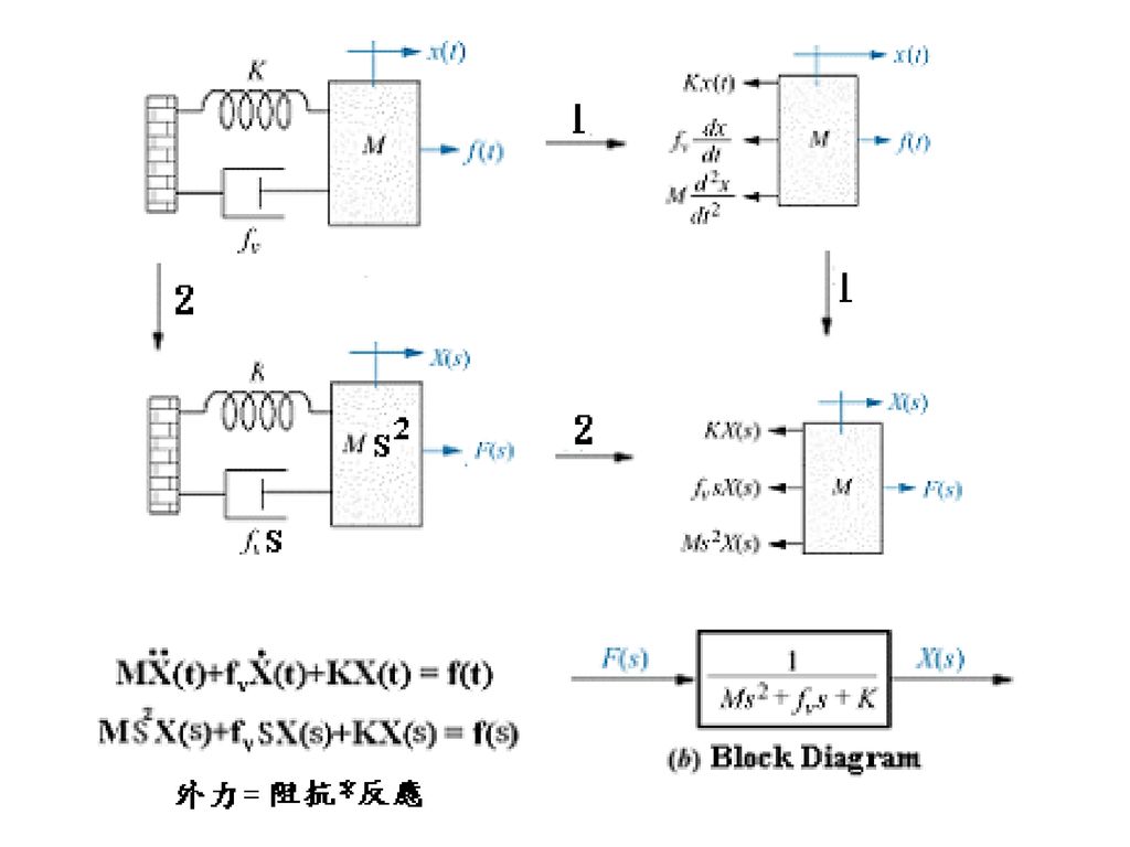
外力 = Σ阻抗 * 反應 F(s) = (MS2+fvS+K) X(s) -MSv(s)-fvv(s)-Kv(s)/S+F(s) = 0 v(s) = SX(s) -MS2X(s)-fvSX(s)-K X(s)+F(s) = 0 MS2X(s)+fvSX(s)+K X(s)= F(s)
 = (MS2+fvS+K) X(s) -MSv(s)-fvv(s)-Kv(s)/S+F(s) = 0 v(s) = SX(s) -MS2X(s)-fvSX(s)-K X(s)+F(s) = 0 MS2X(s)+fvSX(s)+K X(s)= F(s)")
116
§ 2.10 Nonlinearities Figure 2.45 a. Linear system;
b. nonlinear system Figure 2.46 Some physical nonlinearities

117
§ 2.11 Linearization Taylor series (非線性系統線性化的工具)
Example Linearization of f(x) about x = /2 where f(x)= 5 cos x. Taylor series (非線性系統線性化的工具) f(x)= f(x0) + (df/dx) x=xo(x-x0)/1! + (d2f/dx2) x=xo(x-x0)2/2! (2.181) f(x0) = f(/2 ) = 5 cos /2 = 0 (df/dx) x=xo(x-x0)/1! = (-5 sin /2) x = -5 x f(x)= -5 x = -5 (x-/2) 直線公式 當 x around x = /2 時為真 Figure Example Linearization of 5 cos x about x = /2
 about x = /2 where f(x)= 5 cos x. Taylor series (非線性系統線性化的工具) f(x)= f(x0) + (df/dx) x=xo(x-x0)/1! + (d2f/dx2) x=xo(x-x0)2/2! (2.181) f(x0) = f(/2 ) = 5 cos /2 = 0. (df/dx) x=xo(x-x0)/1! = (-5 sin /2) x = -5 x. f(x)= -5 x = -5 (x-/2) 直線公式 當 x around x = /2 時為真. Figure 2.48 Example 2.26 Linearization of 5 cos x about x = /2.")
118
Skill assessment exercise

119
Skill assessment exercise

120
Skill assessment exercise

121
Skill assessment exercise

122
Skill assessment exercise

Similar presentations


 Analog.>")


 泉州六中 苏碧贤.>")
 的系統,其機率分別為 (P(x1),P(x2)) 計算當 (P(x1),P(x2)) 分別為 : (0, 1) 、 (0.1, 0.9) 、 (0.2, 0.8) 、 (0.3, 0.7) 、 (0.4, 0.6) 、 (0.5,>")


 报告人:詹道友 (合肥八中).>")


 與電樞繞組 (armature.>")


>")