The Greedy Method.

Presentation on theme: "The Greedy Method."— Presentation transcript:

1 The Greedy Method

2 Outline Introduction – Lee’s MST – Lee’s and mine
Kruskal’s algorithm Prim’s algorithm Huffman Code – Cormen’s Knapsack Problem – Lee’s and Cormen’s Shortest Path Algorithms – Mine

3 The Greedy Method Suppose that a problem can be solved by a sequence of decisions. The greedy method has the property that each decision is locally optimal. These locally optimal solutions will finally add up to be a globally optimal solution. Only a few optimization problems can be solved by the greedy method.

4 The Greedy Method E.g. Pick k numbers out of n numbers such that the sum of these k numbers is the largest. Algorithm: FOR i = 1 to k pick out the largest number and delete this number from the input. ENDFOR

5 The Greedy Method E.g. Find a shortest path from v0 to v3.
The greedy method can solve this problem. The shortest path: = 7.

6 The Greedy Method E.g. Find a shortest path from v0 to v3 in the multi-stage graph. Greedy method: v0v1,2v2,1v3 = 23 Optimal: v0v1,1v2,2v3 = 7 The greedy method does not work. This is because it never looks ahead.

7 Minimal Spanning Trees
It may be defined on Euclidean space points or on a graph. G = (V, E): weighted connected undirected graph Spanning tree : S = (V, T), T  E, S is a undirected tree Minimal spanning tree (MST) : a spanning tree with the smallest total weight.

8 Minimal Spanning Trees
A graph and one of its minimum spanning trees (MSTs)

9 圖的最小含括樹(MST) 一個最小含括樹演算法  Kruskal演算法，採用貪婪法(greedy method)的策略來建構最小含括樹，也就是每次都是挑選最小成本且不形成cycle的邊加入最小含括樹T之中，如此經過n-1次的邊的挑選之後形成的累積成本必定是最小。 另一個Prim演算法所採用的策略稱為貪婪法(greedy method)，也就是每次都是挑選最小成本的邊加入最小含括樹T之中，經過n-1次的挑選之後形成的累積成本必定是最小。由於每次挑選邊時，都是挑選一個具有連結X及V-X的邊，也就是說挑一個一頂點在X，而另一個頂點在V-X的邊，因此，將所挑選的邊加入T之後不會形成循環(cycle)，這代表T是一棵樹(tree)。

10 Kruskal’s algorithm for finding MST
Step 1: Sort all edges Step 2: Add the next smallest weight edge to the forest if it will not cause a cycle. Step 3: Stop if n-1 edges. Otherwise, go to Step2.

11 Kruskal’s Algorithm Algorithm Kruskal(G)
Input：G=(V, E)為無向加權圖(undirected weighted graph)，其中V={v0,…,vn-1} Output：G的最小含括樹(minimum spanning tree, MST) T← //T為MST，一開始設為空集合 while T包含少於n-1個邊 do 選出邊(u, v)，其中(u, v)E，且(u, v)的加權(weight)最小 E←E-(u, v) if ( (u, v)加入T中形成循環(cycle) ) then 將(u, v)丟棄 else T←T(u, v) return T

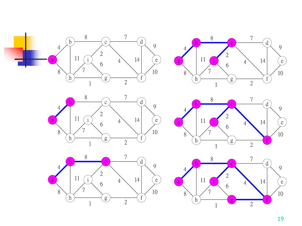
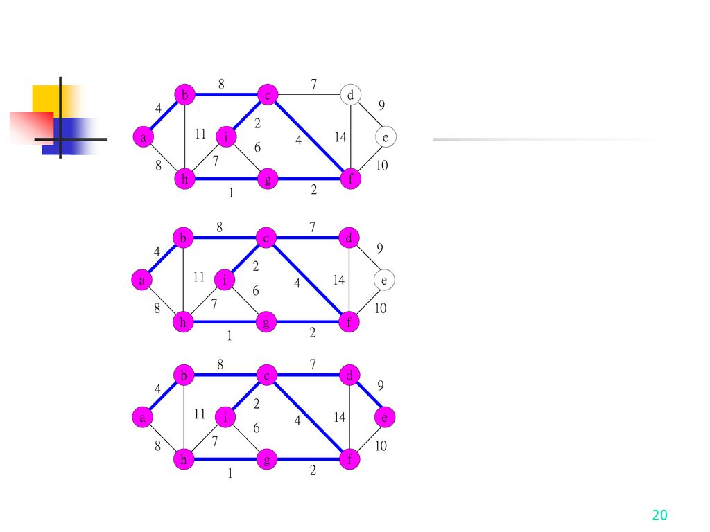
12 Kruskal’s Algorithm -Construct MST

13

14 a c i g f e d h b 8 4 11 7 1 14 10 9 2 6

15 8 7 b c d 4 9 2 a 11 i 4 14 e 6 7 8 10 h g f 1 2 8 7 b c d 4 9 2 a 11 i 4 14 e 6 7 8 10 h g f 1 2

16 Kruskal’s Algorithm - Construct MST
How do we check if a cycle is formed when a new edge is added? By the SET and UNION method. A tree in the forest is represented as a SET. If (u, v)  E and u, v are in the same set, then the addition of (u, v) will form a cycle. If (u, v)  E and uS1 , vS2 , then perform UNION of S1 and S2 .

17 Time complexity for Kruskal’s algorithm
Time complexity: O(|E| log|E|) Sorting : O(|E| log|E|) Finding Element in a set O(|E| log|E|) : O(|E| ) |E|=n2 in the worst case Union two sets By amortized analysis O(n2 log n)

18 Prim’s algorithm Algorithm Prim(G)
Input：G=(V, E)為無向加權圖(undirected weighted graph)，其中V={v0,…,vn-1} Output：G的最小含括樹(minimum spanning tree, MST) T← //T為MST，一開始設為空集合 X←{vx} //隨意選擇一個頂點vx加入集合X中 while T包含少於n-1個邊 do 選出(u, v)E，其中uX且vV-X，且(u, v)的加權(weight)最小 T←T(u, v) X←X{v} return T

19

20

21 Time complexity for Prim’s algorithm
Outter loop: n-1  O(n) Inner loop: choose minimal weight (u, v) for u in X and v in V-X.  O(n) (by using two vecters C1 and C2 propose by Prim) Time complexity: O(n2) If |E|<<n2 then adopt Kruskal’s algorithm.

22 Using an adjacency matrix to represent a graph

23 16.3 Huffman codes a b c d e f Frequency (in hundred) 45 13 12 16 9 5 Fixed length codeword 000 001 010 011 100 101 Variable length codeword 111 1101 1100 Prefix code: no codeword is also a prefix of some other codeword.

24 Can be shown that the optimal data compression achievable by a character code can always be achieved with prefix codes. Simple encoding and decoding. An optimal code for a file is always represented by a binary tree.

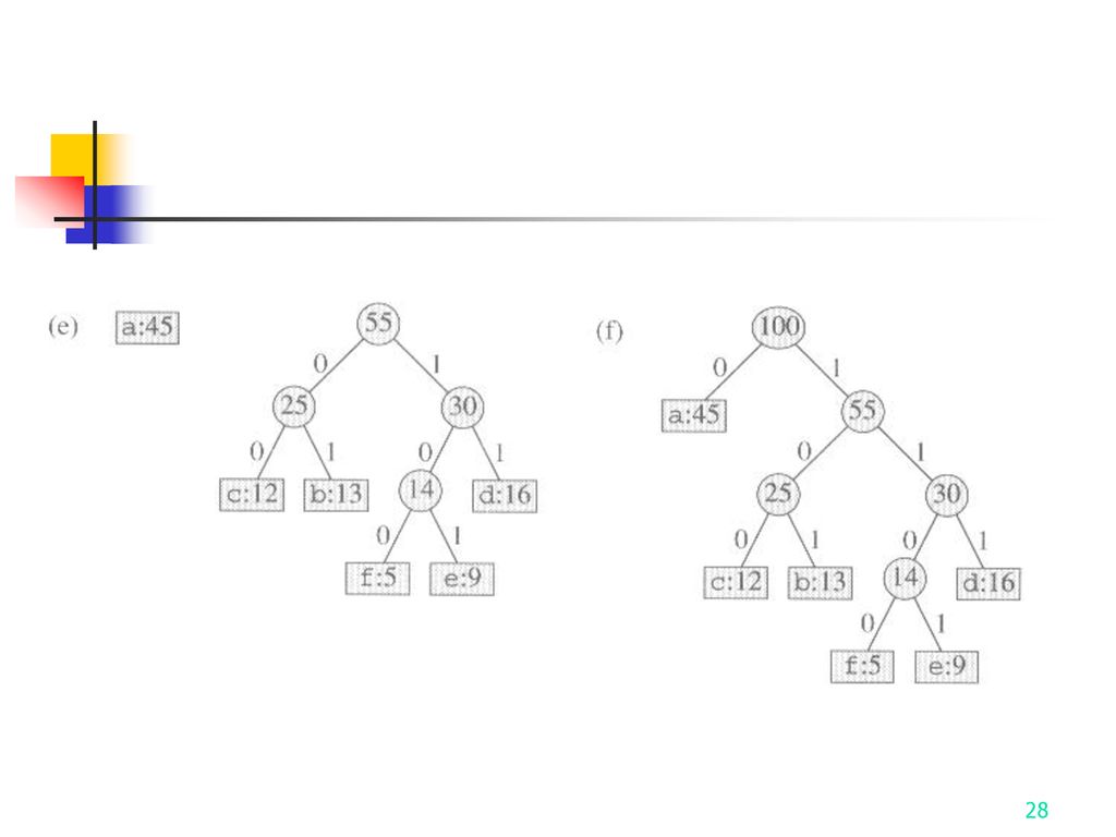
25 Tree correspond to the coding schemes

26 Constructing a Huffman code
2 Q  C 3 for i  1 to n – 1 4 do allocate a new node z left[z]  x  EXTRACT-MIN(Q) right[z]  y  EXTRACT-MIN(Q) f[z]  f[x] + f[y] INSERT(Q,z) 9 return EXTRACT-MIN(Q) Complexity: O(n log n)

27 The steps of Huffman’s algorithm

28

29 The knapsack problem n objects, each with a weight wi > 0
a profit pi > 0 capacity of knapsack: M Maximize Subject to 0  xi  1, 1  i  n

30 The knapsack problem The greedy algorithm:
Step 1: Sort pi/wi into non-increasing order. Step 2: Put the objects into the knapsack according to the sorted sequence as much as possible.

31 The knapsack problem E.g. n = 3, M = 20, (p1, p2, p3) = (25, 24, 15)
(w1, w2, w3) = (18, 15, 10) Sol: p1/w1 = 25/18 = 1.32 p2/w2 = 24/15 = 1.6 p3/w3 = 15/10 = 1.5 Optimal solution: x1 = 0, x2 = 1, x3 = 1/2

32 The greedy strategy does not work for the 0-1 knapsack

33 圖的最短路徑 由圖(graph)中的某個頂點(vertex)v到圖中的另一頂點u，若v到u之間存在一條路徑(path)，則路徑中所經過的邊(edge)的加權值(weight)的總合稱為路徑的成本(cost)。所有路徑中具有最小成本的稱為最短路徑(shortest path)。 由於最短路徑具有許多應用，因此有許多求取最短路徑的演算法，以下我們介紹最有名的幾個演算法：(1). Dijkstra演算法(Dijkstra Algorithm) (2). Bellman-Ford演算法(Bellman-Ford Algorithm)及(3). All Pair Shortest Path Algorithm。

34 The single-source shortest path problem
Graph and shortest paths from v0 to all destinations

35 圖的最短路徑 Dijkstra演算法: Dijkstra演算法屬於求取單一來源(source)至所有目標(destination)頂點的一至多(one-to-all)最短路徑演算法

36 圖的最短路徑 我們將d[u]以加中括號的方式標記在每一個頂點旁，使用圖8-5來說明Dijkstra演算法求頂點A到每一個頂點最短路徑的過程。
若要讓Dijkstra演算法也能夠求出每一條最短路徑所經過的每一個頂點，則我們要將每一頂點在最短路徑中的前一頂點紀錄下來，其作法為增加一個陣列p(代表predecessor，前行者)來記錄最短路徑中的每一個頂點的前一頂點。並將Dijkstra演算法之if敘述修改如下： if (d[u]+w[u][x]<d[x]) then d[x]←d[u]+w[u][x] p[x]←u //此敘述為新加入者，代表在最短路徑中頂點ｘ的前一頂點為ｕ

37 圖8-5

38 圖8-5

39 圖的最短路徑 以下我們以表8-1來說明Dijkstra演算法的執行過程：

40 圖的最短路徑 Bellman-Ford演算法也是屬於求取單一來源至所有目標頂點的演算法，與Dijkstra演算法不同的是，Bellman-Ford演算法可以在具有負加權(negative weight)的圖上也正確的求出一到多(one-and-all)的最短路徑。以下是Bellman-Ford演算法：

41 圖的最短路徑 Bellman-Ford演算法的精神是在第一次迴圈執行時即求出所有”1-邊路徑(one-edge path)”的最短路徑，而在第二次迴圈執行時即求出所有”2-邊路徑(two-edge path)” 的最短路徑，…依此類推。 Floyd-Warshall演算法利用一個n×n(n為頂點總數)二維成本(cost)陣列c來記錄每一組頂點配對間的最短路徑成本，在啟始(initial)狀況時，c[i][i]=w[i][j]，for each i and j。而當Floyd-Warshall演算法執行時會不斷的更新陣列c。 在第k次更新陣列c時，表示c中所紀錄的最短路徑是經由編號小於或等於k的頂點所造成的。因此，當第n次更新陣列c時，則表示c中所紀錄的最短路徑是經由所有頂點所造成的，這也就完成演算法所需求取的結果。

42 圖的最短路徑 Floyd-Warshall的所有頂點對最短路徑(all-pair shortest path)演算法：

43 圖的最短路徑 以下我們在圖8-6中使用圖8-5中的圖(graph)來說明Floyd-Warshall的所有頂點對最短路徑演算法執行過程，請注意，我們使用代表在啟始狀況之值，代表在迴圈第一次，第二次，…，及第k次執行時陣列c的值。

44 圖8-6

45 圖8-6

46 The End