Continuous Probability Distributions

Presentation on theme: "Continuous Probability Distributions"— Presentation transcript:

1 Continuous Probability Distributions
第六章 連續機率分配 Continuous Probability Distributions

2 機率分配 離散型機率 分配 (教材第5章) 連續型機率分配 不同隨機變數值的機率分佈狀況
用來 描述 不同隨機變數值的機率分佈狀況 How probabilities are distributed over the values of the random variable. 分為 離散型機率 分配 (教材第5章) 連續型機率分配

3 連續型機率分配 Continuous Probability Distribution 機率密度函數 特定區間面積
其函數稱 機率密度函數 Probability Density Function 機率值為 特定區間面積 條件

4 Uniform Probability Distribution
教材6.1 均勻(矩形)機率分配 Uniform Probability Distribution Consider the random variable x representing the flight time of an airplane traveling from Chicago to New York. Suppose the flight time can be any value in the interval from 120 minutes to 140 minutes. Let us assume that sufficient actual flight data are available to conclude that the probability of a flight time with every 1-minute interval being equally likely.

5 Uniform Probability Distribution
均勻(矩形)機率分配 Uniform Probability Distribution f (x)= 1/ for 120≦x≦140 elsewhere f (x) 1/20 x 120 125 130 135 140 Flight Time in Minutes

6 均勻(矩形)機率分配 f (x)= 1 b - a 特性： 隨機變數在任何區間的機率皆相同
Uniform Probability Density Function 1 for a ≦ x ≦ b b - a f (x)= (6.1) elsewhere

7 Area as a Measure of Probability
Consider the area under the graph of f (x) in the interval from 120 to 130. The area is rectangular ,and the area of a rectangle is simply the width multiplied by the height. f (x) P(120≦x≦130)=Area=1/20(10)=.50 1/20 10 x 120 125 130 135 140 Flight Time in Minutes

8 We talk about the probability of the random variable assuming a value within some given interval instead of a particular value. The probability of the random variable assuming a value within some given interval from x1 to x2 is defined to be the area under the graph of the probability density function between x1 and x2 . The probability of a continuous random variable assuming any particular value exactly is zero.

9 The Expected Value and Variance of Uniform Continuous Probability
期望值 變異數 a is the smallest value and b is the largest value that the random variable may assume

10 Normal Probability Distribution
教材6.2 常態機率分配 Normal Probability Distribution Normal Curve → bell-shaped 鐘型分配(左右對稱) Standard Deviation σ x μ Mean

11 Normal Probability Density Function
(6.2) where μ=mean σ=standard deviation π= e =

12 The characteristics of the normal distribution
1. The entire family of normal distribution is differentiated by its mean μ and its standard deviation σ. 不同平均數及標準差形成不同常態分配 2. The highest point on the normal curve is at the mean ,which is also the median and mode of the distribution. 最高點為平均數，平均數等於中位數等於眾數

13 3. The mean of the distribution can be any numerical value : negative ,zero ,or positive. Three normal distributions with the same standard deviation but three different means (-10 , 0 ,and 20) are shown here. 平均數可以是任意數值 x -10 20

14 4.The normal distribution is symmetric ,with the shape of the curve to the left of the mean a mirror image of the shape of the curve to the right of the mean. The tail of the curve extend to infinity in both directions and theoretically never touch the horizontal axis. Because it is symmetric ,the normal distribution is not skewed ;its skewness measure is zero. 是對稱分配，以平均數為對稱中心

15 5. The standard deviation determines how flat and wide the curve is
5. The standard deviation determines how flat and wide the curve is. Larger values of the standard deviation result in wider ,flatter curves , showing more variability in the data. 標準差較大則曲線較寬，資料較分散 σ=5 σ=10 x μ

16 6.Probabilities for the normal random variable are given by areas under the curve. The total area under the curve for the normal distribution is 1. Because the distribution is symmetric ,the area under the curve to the left of the mean is .50 and the area under the curve to the right of the mean is .50. 曲線下面積為1

17 7.The percentage of values in some commonly used intervals are :
(a) 68.3% of the values of a normal random variable are within plus or minus one standard deviation of its mean. (b) 95.4% of the values of a normal random variable are within plus or minus two standard deviation of its mean. (c) 99.7% of the values of a normal random variable are within plus or minus three standard deviation of its mean.

18 99.7% 95.4% 68.3% x μ µ-3σ µ-2σ µ-1σ µ+1σ µ+2σ µ+3σ

19 Standard Normal Probability Distribution 標準常態分配
A random variable that has a normal distribution with a mean of zero and a standard deviation of one is said to have a standard normal probability distribution. The letter z is commonly used to designate this particular normal random variable. 轉換標準→ z = σ=1 X -μ σ x μ=0

20 Standard Normal Density function
1 -z²/2 f (x) = e √̅ 2π

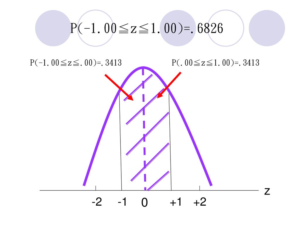
21 P(.00≦z≦1.00)=.3413 z 1

22 查表 z .00 .01 .02 . .9 1.0 1.1 1.2 .3159 .3186 .3212 .3413 .3438 .3461 .3643 .3665 .3686 .3849 .3869 .3888 P(.00≦z≦1.00)

23 P(-1.00≦z≦1.00)=.6826 z -2 -1 +1 +2 P(-1.00≦z≦.00)=.3413
+1 +2

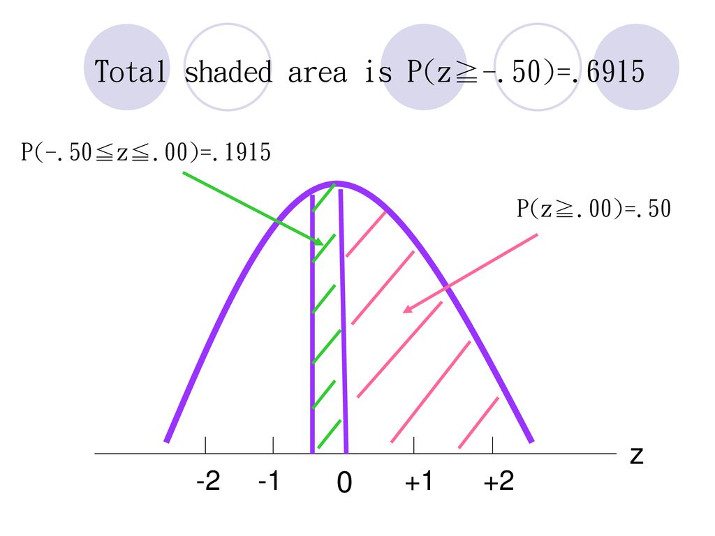
24 z -3 -2 -1 +1 +2 +3 .5 of total area is to the right of z=0
.5 of total area is to the left of z=0 .4429 is the area between z=0 and z=1.58 P(z≧1.58)= =.0571 z -3 -2 -1 +1 +2 +3

25 Total shaded area is P(z≧-.50)=.6915
-2 -1 +1 +2

26 P(0≦z≦1.00)=.3413 P(0≦z≦1.58)=.4429 P(1≦z≦1.58)=.1016 z -2 -1 +1 +2

27 Probability or area .10 z -3 -2 -1 +1 +2 +3 What is this z value ?

28 0.4 0.1 z -3 -2 -1 +1 +2 +3 What is this z value ?

29 查表 z … .07 .08 .09 1.0 1.1 1.2 1.3 … .3557 .3559 .3621 .3790 .3810 .3830 .3980 .3997 .4015 .4147 .4162 .4177 … Area value in body of table closest to The probability is approximately .10 that the z value will be larger than 1.28.

30 Converting to the Standard Normal Distribution
X -μ z = (6.3) σ Example ： μ=10 σ=2 What is the probability that the random variable x is between 10 and 14 ?

31 Converting to the Standard Normal Distribution
X = 10 Z = (10-10)/2 = 0 X=14 Z = (14-10)/2 = 2 →The probability of x being between 10 and 14 is given by the equivalent probability that z is between 0 and 2 for the standard normal distribution =.4772.

32 Grear Tire Company Problem
Suppose the Grear Tire Company developed a new steel-belted radial tire ,and managers believe that the mileage guarantee offered with the tire will be an important factor in the acceptance of the product. The Grear`s managers want probability information about the number of miles the tires will last.

33 Grear Tire Company Problem
From actual road tests with the tires , Grear`s engineering group estimates： μ=36,500 σ=5,000 The data collected indicate a normal distribution is a reasonable assumption. What percentage of the tires can be expected to last more than 40,000 miles? (What is the probability that the tire mileage will exceed 40,000?)

34 Grear Tire Company Problem
At X=40,000 ,we have z = (x -μ) /σ = (40,000-36,500)/5,000 =.70

35 σ=5,000 P(x≧40,000)=? x 40,000 μ=36,500 z .70 Z=0 corresponds to x=μ=36,500 Z=.70 corresponds to x=40,000

36 σ=5,000 P(x≧40,000) = =.2420 .2580 x 40,000 μ=36,500 z .70 Z=0 corresponds to x=μ=36,500 Z=.70 corresponds to x=40,000

37 Grear Tire Company Problem
σ=5,000 10% of tires eligible for discount guarantee x μ=36,500 Guarantee mileage=?

38 x z Z=-1.28 0.4 σ=5,000 10% of tires eligible for discount guarantee
μ=36,500 z Z=-1.28

39 Grear Tire Company Problem
To find the value of x corresponding to z=1.28 ,we have X -μ → X =μ-1.28σ z = =-1.28 σ With μ=36,500 and σ=5,000 X = 36, (5,000) = 30,100 A guarantee of 30,100 miles will meet the requirement that approximately 10% of the tires will be eligible for the guarantee.

40 Normal Approximation of Binomial Probabilities
教材6.3 Normal Approximation of Binomial Probabilities In case where the (1)number of trials is greater than 20 (2)np≥5 (3)n(1-p) ≥5 , the normal distribution provides an easy-to-use approximation of binomial probabilities. μ=np σ= np(1-p)

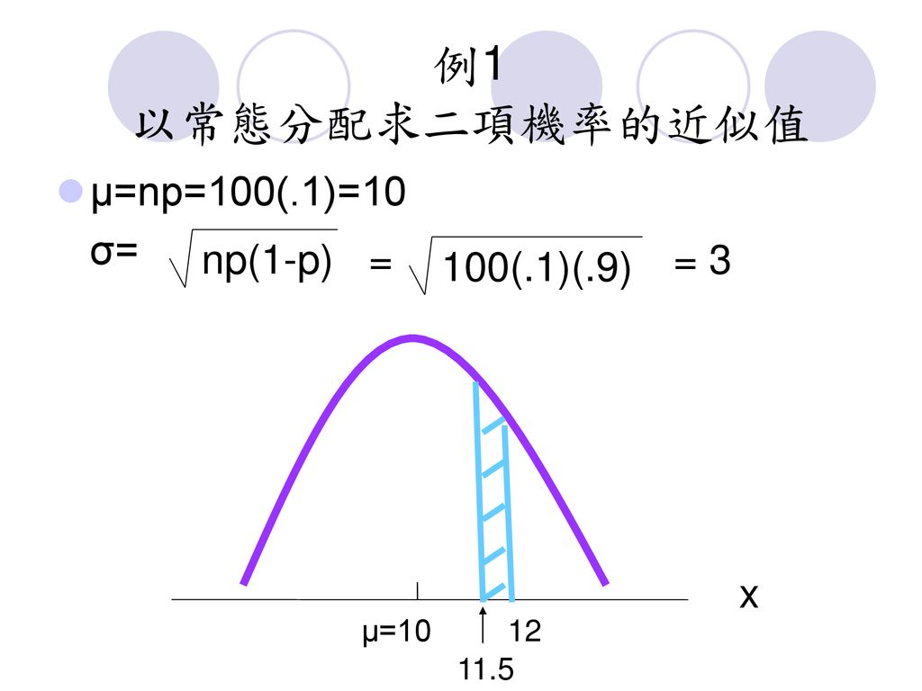
41 例1 以常態分配求二項機率的近似值 Suppose a particular company has a history of making errors in 10% of its invoices. A sample of 100 invoices has been taken ,and we want to compute the probability that 12 invoices contain errors. That is ,we want to find the binomial probability of 12 successes in 100 trials.

42 例1 以常態分配求二項機率的近似值 離散的二項機率分配值P(x=12)，可以用連續的常態分配的f(11.5≦x≦12.5) 來近似之。
由12加減的0.5稱為連續校正因子(continuity correction factor)。

43 例1 以常態分配求二項機率的近似值 μ=np=100(.1)=10 σ= np(1-p) = = 3 100(.1)(.9) x μ=10
12 11.5

44 例1 以常態分配求二項機率的近似值 z = z = 將常態分配轉換成標準常態分配以計算f(11.5≦x≦12.5)： 12.5 – 10
=0.83 σ 3 X -μ 11.5 – 10 x=11.5 z = = =0.50 σ 3 f(11.5≦x≦12.5) = f(0.5≦z≦0.83) = =

45 例2 以常態分配求二項機率的近似值 z = 求100張發票中，13張(含)以下有錯誤的機率。 使用連續校正因子，以13.5來求近似機率。
X -μ =1.17 z = = 3 σ

46 例2 以常態分配求二項機率的近似值 f (x≦13.5) = f (z≦1.17) = 0.379 + 0.5 = 0.879 x μ=10

47 Exponential Probabilities Distribution指數機率分配
教材6.4 Exponential Probabilities Distribution指數機率分配 一個常被用來描述完成工作所需時間的連續機率分配是指數機率分配。 例：車輛到達洗車廠的時間間隔、貨車裝貨時間、公路路面損壞的間隔距離。 指數機率密度函數 f (x) = -x/μ 1 (6.4) e for x≧0 μ≧0 μ

48 例子 指數機率分配：Schips 碼頭 假定X = 在 Schips 碼頭裝滿一卡車貨物所需的時間 X是指數分配
平均裝貨時間為15分鐘(μ=15) 其機率密度函數為 f (x) = -x/15 1 e 15

49 例子 指數機率分配：Schips 碼頭 Figure 6.10 f(x) 0.07 0.05 0.03 0.01 x 5 15 25 35
5 15 25 35 45 裝貨時間

50 計算指數分配機率的分法 分配曲線下的區段面積決定隨機變數在某範圍內的機率。 在 Schips 碼頭的例子中
裝貨時間少於6分鐘的機率(X≦6)是圖6.10中X=0到X=6間的曲線下面積 裝貨時間少於18分鐘的機率(X≦18)是X=0到X=18間的曲線下面積 裝貨時間為6分鐘到18分鐘(6≦X≦18)的機率是計算X=6到X=18間的曲線下面積

51 計算指數分配機率的分法 利用下列公式來計算指數隨機變數在小於等於某一特定X值(以X0表示)下的機率。 指數分配：累積機率
(Cumulative Probabilities) P(X≦X0) = 1- -x0/μ e (6.5)

52 計算指數分配機率的分法 e e e 在 Schips 碼頭的例子中，X=裝貨時間且μ=15，因此： P(X≦X0) = 1-
裝貨時間介於6分鐘到18分鐘的機率等於 =0.3691 -x0/15 e -6/15 e -18/15 e

53 計算指數分配機率的分法 Figure 6.11裝貨時間少於6分鐘的機率或面積 f(x) P(X≦6)=0.3297 x 裝貨時間 0.07
0.06 0.05 0.04 0.03 0.02 0.01 x 5 10 15 20 25 30 35 40 裝貨時間

54 計算指數分配機率的分法 指數分配的特徵之ㄧ是：平均數=標準差 在 Schips 碼頭的例子中，裝貨所需平均時間為μ=15分鐘
因此，裝貨時間的標準差σ=15分鐘 變異數為σ²=15²=225

55 卜瓦松分配與指數分配的關係 卜瓦松機率函數 f (x) = 其中 μ=某段區間內的平均發生次數
其中 μ=某段區間內的平均發生次數 如果卜瓦松分配適合用來表示某一區間內的事件發生次數的的機率，指數分配就可以描述二次事件發生的時間間隔的機率。 x -μ μ e x !

56 卜瓦松分配與指數分配的關係 假設洗車廠的來車數量呈卜瓦松分配，平均每小時10輛汽車，則以X表示來車車數的卜瓦松機率分配函數是：
f (x) = 連續到達的兩輛汽車之時間間隔為： 1小時/10輛車 = 0.1 小時/車(μ=0.1) 因此，對應的指數機率密度函數為 f (x) = =10 x -10 10 e x ! 1 -x/0.1 -10x e e 0.1