Chapter 7 The Laplace Transform

Presentation on theme: "Chapter 7 The Laplace Transform"— Presentation transcript:

1 Chapter 7 The Laplace Transform
作用：把微分變成乘法 Chapter 4 曾經提過 可寫成 Laplace transform可以將 變成

2 Section 7-1 Definition of the Laplace Transform
Definitions  Laplace Transform of f(t) 經常以大寫來代表 transform 的結果

3 Laplace Transform is one of the integral transform
把一個 function 變成另外一個 function  integral transform: 可以表示成積分式的 transform  kernel 對 Laplace transform 而言 a = 0, b   註：Chap. 14 將教到的 Fourier transform, 也是一種 integral transform

4 Linear Property 事實上，所有的 integral transform 都有linear property

5 7-1-3 The Laplace Transforms of Some Basic Functions
f(t) F(s) 1 t n exp(at) sin(kt) cos(kt) sinh(kt) cosh(kt) (彼此密切相關）

6 Example 1 (text page 280) (1) 比較正式的寫法是 (2) 這裡假設 Re(s) > 0, 所以

7 Example 2 (text page 280)

8 Example 3 (text page 280) stable Pole (分母為0 的地方) 在複數平面左半邊 unstable Pole 在複數平面右半邊 Im(s) Re(s) s = -3

9 Example 4 (text page 281) 除了課本的解法之外， 另一個解法 Example (text page 281)

10 7-1-4 When Does the Laplace Transforms Exist?
Constraint 1 for the existence of the Laplace transform : For a function f(t), there should exist constants c, M > 0, and T > 0 such that for all t > T In this condition, f(t) is said to be of exponential order c Fig

11 Example： f(t) = t, e−t, 2cost 皆為 exponential order 1
Fig (a) (b) (c) 補充：其實，對一個function 而言， exponential order c 不只一個 例子： f(t) = tn 為 exponential order c, c > 0 There exists an M such that if c > 0

12 Example： f(t) = exp(t2) 時，並不存在一個 c 使得
for all t > T Fig 只要有一個 c 使得 for all t > T 我們稱 f(t) 為 of exponential order 否則，我們稱 f(t) 為 not of exponential order

13 Constraint 2 for the existence of the Laplace transform :
f(t) should be piecewise continuous on [0, ) 在任何 t  [a, b] 的區間內 (0  a  b < ) f(t) 為 discontinuous 的點的個數為有限的 稱作是「piecewise continuous」 Fig 注意： 1/t 不為 piecewise continuous

14 Constraints 1 and 2 are “sufficient conditions”
若滿足 Laplace transform 存在 若不滿足 Laplace transform 未必不存在

15 反例： f(t) = t−1/2 不為 piecewise continuous
但是 Laplace transform 存在 補充說明： f(t) = t−1/2 不為 piecewise continuous 是因為 f(0)   所以 f(t) 在 t = 0 附近有無限多個不連續點 事實上，只要 f(t1)  , |t1| is not infinite， f(t) 必定不為 piecewise continuous

16 Theorem 7.1.3 If f(t) is piecewise continuous on [0, ) and of exponential order, then

17 Section 7-1 需要注意的地方 (1) Laplace transform of some basic functions 要背起來 (2) 記公式時，一些地方要小心 sin, sinh, 1/tn 沒有平方 sin kt 有平方 (3) 熟悉(a) 包含 exponential function 的積分 以及 (b) 的積分技巧 (4) 要迅速判斷一個式子當 t  時是否為 0 (5) 小心正負號

18 附錄七：充分條件和必要條件的比較 If A is satisfied, then B is also satisfied :
A is the sufficient conditions of B (充分條件) A B If B is satisfied, then A is bound to be satisfied : A is the necessary conditions of B (必要條件) B A B is satisfied if and only if A is be satisfied : A is the necessary and sufficient conditions of B (充分且必要的條件)

19 Section 7-2 Inverse Transforms and Transforms of Derivatives
本節有兩大部分： (1) inverse Laplace transform 的計算 (7-2-1 ~ 7-2-3) (2) 將微分變成 Laplace transform 當中的乘法 (7-2-4 ~ 7-2-6)

20 7-2-1 Inverse 方法一： One-to-One Relation
When (1) f1(t) and f2(t) are piecewise continuous on [0, ), and (2) f1(t) and f2(t) are of exponential order, then if f1(t)  f2(t) then F1(s)  F2(s) 換句話說，在這種情形下，Laplace transform 是 one-to-one 的運算。 If the Laplace transform of f1(t) is F1(s), then the inverse Laplace transform of F1(s) must be f1(t).

21 Table of Inverse Laplace Transforms
F(s) f(t) = L−1{F(s)} 1 t n exp(at) sin(kt) cos(kt) sinh(kt) cosh(kt)

22 Example 1 (text page 287) (a) Example 2 (text page 287)

23 7-2-2 Inverse 方法 (二） Decomposition of Fractions
Example 3 (text page 288) 問題：A, B, C 該如何算出？ 太麻煩

24 7-2-3 計算分數分解係數的快速法 兩邊各乘上 (s − 1) 這二個步驟可以合併 把 s = 1 代入
計算分數分解係數的快速法 兩邊各乘上 (s − 1) 這二個步驟可以合併 把 s = 1 代入 左式乘上 (s − 2)後，把 s = 2 代入 左式乘上 (s + 4)後，把 s = −4 代入

25 (Cover up method) 通則：要將一個 fraction 分解 a1, a2, …., aN 互異 (1) 用多項式的除法算出 Q(s) 商 餘式 使得 order of K1(s) < N (2) 算出 An

26 例子： Q(s) = 1

27

28  小技巧：其實，如果只剩下一個未知數，我們可以將 s 用某個數代入， 快速的將未知數解出

29 例子：

30 7-2-4 Transforms of Derivatives

31 Theorem 7.2.2 Derivative Property of the Laplace Transform

32 7-2-5 Solving the Constant Coefficient Linear DE by Laplace Transforms

33 (auxiliary)

34 G(s): Laplace transform of the input
Q(s): caused by initial conditions Y(s): Laplace transform of the response W(s): transform function L−1[W(s)Q(s)]: zero-input response or state response L−1[W(s)G(s)]: zero-state response or input response

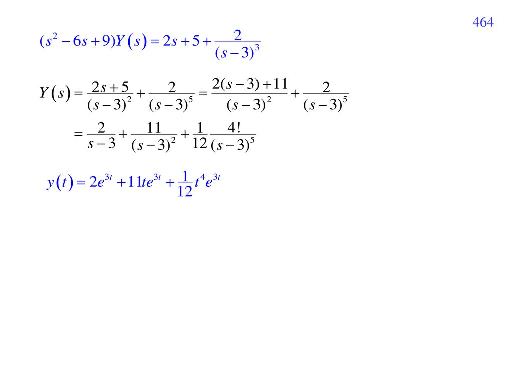
35 Example 4 (text page 290) (Step 1) Laplace Transform (Step 2) Decompose (Step 3) Inverse Laplace Transform

36 Example 5 (text page 291) 快速法 (Step 1) Laplace (Step 2) Decompose (Step 3) Inverse

37 快速法 (A) 求 P(s) 很像 Sec. 4-3 的… (B) 求 Q(s)

38 相加 例如，page 454的例子 Q(s)

39 7-2-7 Section 7.2 需要注意的地方 (1) 熟悉分數分解 (2) 可以簡化運算的方法，能學則學
鼓勵各位同學多發揮創意，多多研究能簡化計算的快速法 數學上…….並沒有標準解法的存在 (3) Derivative 公式 initial conditions 的順序別弄反

40 Section 7-3 Operational Properties I
介紹兩個可以簡化 Laplace transform 計算的重要性質 First Translation Theorem (translation for s) Second Translation Theorem (translation for t) u(t): unit step function (注意兩者之間的異同)

41 7-3-1 First Translation Theorem (Translation for s)
Proof:

42 7-3-1-1 Inverse of “Translation for s”
When f(t) is piecewise continuous and of exponential order (一對一) 註： Sections 7-3 和 7-4 其他的定理亦如此

43 Examples Example 1 (text page 295) (a) (b)

44 Example 2 (text page 296) (a) (b)

45 Example 3 (text page 297) s Q(s) = +

46

47 7-3-2 Step Function u(t): unit step function u(t) = 1 for t > 0
t-axis t = 0 u(t−a) u(t−a) = 1 for t > a u(t−a) = 0 for t < a t-axis t = a The unit step function acts as a switch (開關).

48  Any piecewise continuous function can be expressed as the unit step function for t  0
Example 5 (text page 298) for 0  t < 5 for t > 5 Fig

49 In general, for 0  t < a for t > a

50 f(t-a)u(t-a) 7-3-3 Second Translation Theorem (Translation for t)
或 a > 0 f(t-a)u(t-a)

51 Proof: 令 t1 = t − a

52 Example 7(a) (text page 300)
Example 8 (text page 300)

53 Example 9 (text page 301) for 0  t <  for t  

54

55 7-3-4 本節需要注意的地方 (1) 套用 “translation for t” 的公式時，
本節需要注意的地方 (1) 套用 “translation for t” 的公式時， 先將 input 變成 g( t + a ) 再作 Laplace transform (例如 Example 7) (2) Second translation theorem (translation for t) 當 a > 0 時才適用 (3) 套用公式時，注意「順序」

56 Section 7-4 Operational Properties II
Derivatives of Transforms 比較： Laplace 微分 乘 sn Laplace 乘 tn 微分

57 Proof of the Theorem of Derivatives of Transforms:

58 Example 1 (text page 307) 練習：為何

59 7-4-2 Convolution (旋積) Definition of convolution: (標準定義)
When f(t) = 0 for t < 0 and g(t) = 0 for t < 0 , 上方的式子可以簡化為下方的式子

60 Convolution 的物理意義 (重要)
當 Input f() 對 output y(t) 的影響為 g(t−) g(t−) 只和 t 與  之間的差有關 Input f() 對 output y(t) 的影響，決定於 t 與  之間的差

61 例如： f() 是在  這個時間點上太陽照射到某個地方的熱量
g(t-) 可想像成是經過了t- 的時間之後，還未幅射回外太 熱量比例 y(t) 可想像成是溫度

62 7-4-3 Convolution Theorem
Multiplication Convolution Proof: note (A) 見後頁說明 令 t =  +  note (B ) 見後頁說明

63 note (A) 定理： note (B) 積分範圍的改變： Fig

64 Example 3 (text page 308) Compute Example 4 (text page 309) Example 5 (text page 309)

65 Integration (想成 “負一次微分”)

66 Example: Example:

67 7-4-5 Transform of a Periodic Function
Theorem 7.4.3 When f(t + T) = f(t) then Proof: 令 f1(t) = f (t) when 0  t < T f1(t) = otherwise f (t) = f1(t) + f1(t − T) + f1(t − 2T) + f1(t − 3T) + ……………. = f1(t) + f1(t −T)u(t − T) + f1(t −2T) u(t −2T ) + f1(t −3T) u(t −3T ) + …………….

68 L{f (t)} = L{f1(t)} + L{f1(t −T)u(t − T)} +L{ f1(t − 2T)u(t − 2T)}
:

69 Example 8 (text page 314) Square Wave (方波) 的例子 for 0  t < 1 for 1  t < 2 Fig

70

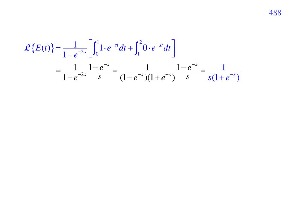
71 Example 9 (text page 314) E(t) 為 page 487 之方波

72 長除法 k = 0, 1, 2, 3, …..

73 的公式 先使用 再算出 註：雖然也可以用 來算 但是較麻煩且容易出錯

74 7-4-6 Section 7.4 要注意的地方 (1) 注意代公式的順序 (例：Page 491 例子)
(2) 熟悉 convolution (3) 變成積分時，別忘了加上 initial value 如 (4) 一定要記熟幾個重要的 properties (7 大性質)

75 Section 7.5 The Dirac Delta Function
Unit Impulse for t < t0−a or t > t0+a for t0−a  t  t0+a 稱作 unit impulse 高= 1/2a 面積 = 1 t0−a t0+a t-axis

76 7-5-2 Dirac Delta Function
for t = t0 for t  t0 Fig

77 7-5-3 Properties of the Dirac Delta Function
(1) Integration (2) Sifting when t0  [p, q] Proof: 當 a 很小的時候，f(t)  f(t0) for t0−a  t  t0+a

78 (3) Laplace transform of (t − t0)
when t0 > 0 Proof: (from the sifting property) (4) Relation with the unit step function

79 Example Example 1(a) (text page 319) 0  t < 2 t  2

80 幾個名詞 where (1) w(t) = L−1{W(s)} 稱作 weight function 或 impulse response Note: When Q(s) = 0 (no initial condition) and G(s) = 1 (g(t) = (t)), Y(s) = W(s), y(t) = w(t). (2) 許多文獻把 Dirac delta function (t − t0) 亦稱作 delta function ， impulse function，或 unit impulse function

81 7-5-6 本節要注意的地方 (1) Dirac delta function 不滿足 Theorem 7.1.3
本節要注意的地方 (1) Dirac delta function 不滿足 Theorem 7.1.3 (2) 幾個定理記熟，本節即可應付自如

82 Section 7-6 Systems of Linear Differential Equations
Chapter 7 的應用題 比較：類似的問題，也曾經在 Section 4-9 出現過 雙彈簧的例子

83 電路學的例子 (由第2, 3 個式子) Fig Fig

84 Example 2 (text page 323) E(t) = 60 V, L = 1 H, R = 50 , C = 10−4 F, i1(t) = i2(t) = 0 ……….. (式1) …... (式2) (式1) × 1 + (式2) × s

85 複習：分子如何算出？ 將 代入式 (1)

86

87 7-6-3 Double Pendulum (雙單擺) 的例子

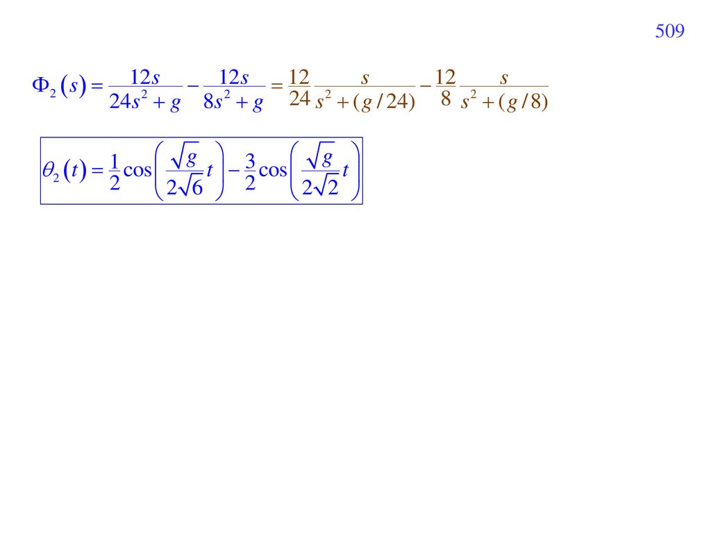
88 Example 3 (text page 324) m1 = 3, m2 = 1, l1 = 12 = 16, 1(0) = 1, 2(0) = 1, '1(0) = 0, '2(0) = 0 Laplace

89 ………….. (式1) ………….. (式2) (式1) × (16s2 + g)  (式2) × 4s2

90 將 代入 (式2) 直接用之前的式子

91

92 分式分解快速驗算技巧 將 s = 0, s = 1, 或其他的值代入，看等號是否成立

93 本節需要注意的地方 (1) 正負號勿寫錯 (2) 要熟悉聯立方程式的變數消去法 (3) 多學習，甚至多「研發」簡化計算的技巧

94 Review of Chapter 7 (1) Laplace transform 定義 Inverse Laplace transform
If and f(t) is piecewise continuous of exponential order then (2) 7 大transform pairs (看講義 page 423)

95 transform pairs 補充 f(t) F(s) tsin(kt) tcos(kt) tsinh(kt) tcosh(kt) u(ta) f (t) = f (t+2a) 1 a b

96 (3) 7 大 properties input Laplace transform (1) Differentiation (Sec 7-2) (2) Multiplication by t (Sec7-4) (3) Integration (Sec 7-4) (續)

97 input Laplace transform (4) Multiplication by exp (Sec7-3) (5.1) Translation (Sec 7-3) (5.2) Translation (Sec 7-3) (6) Convolution (Sec 7-4) (7) Periodic Input (Sec 7-4) f(t) = f(t + T)

98 Properties 補充 input Laplace transform Scaling f(t / a) aF(as) Multiple Integrations Integration for s f(t) / t

99 (4) 簡化運算的方法 分式分解 (see pages ) Initial conditions (see pages 455, 456) (5) Delta function 的四大性質 Pages 495, 496

100 (6) General solutions Laplace transform 的 general solution，可以用 initial conditions 來表示。 用Sec. 4-3 的方法解出 例子： 用 Laplace transform ：

101 和 Section 4-3 的解互相比較 將 代入

102 Exercise for Practice Sec. 7-1: , 8, 9, 18, 32, 33, 36, 38, 41, 49, 54, 55, 56, 57, 58 Sec. 7-2: 　 11, 20, 23, 26, 27, 30, 40, 41, 45, 46, 49 Sec. 7-3: 　 10, 16, 19, 20, 24, 34, 35, 42, 44, 56, 58, 62, 64, 68, , 74, 83 Sec. 7-4: 　 8, 13, 29, 32, 34, 42, 47, 50, 56, 57, 58, 63, 65, 67, 70 Sec. 7-5: 　 5, 6, 8, 11, 12, 17 Sec. 7-6: 　 8, 11, 12, 14, 15 Review 7: 　12, 24, 25, 29, 38, 40, 41, 44, 45, 46